Computing stuff tied to the physical world

Archive for the ‘Software’ Category

Wrapping up

In AVR, Hardware, News, Software, Musings on Oct 6, 2013 at 00:01

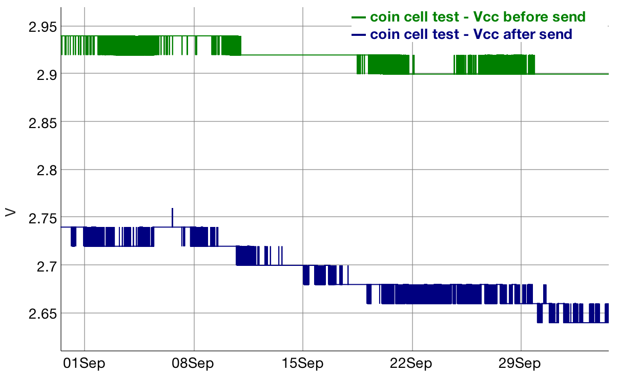
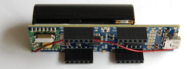
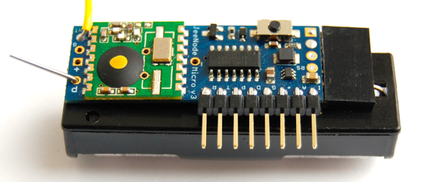
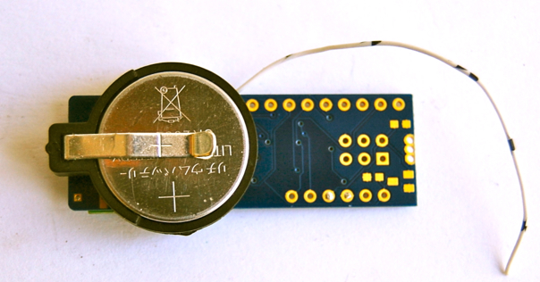
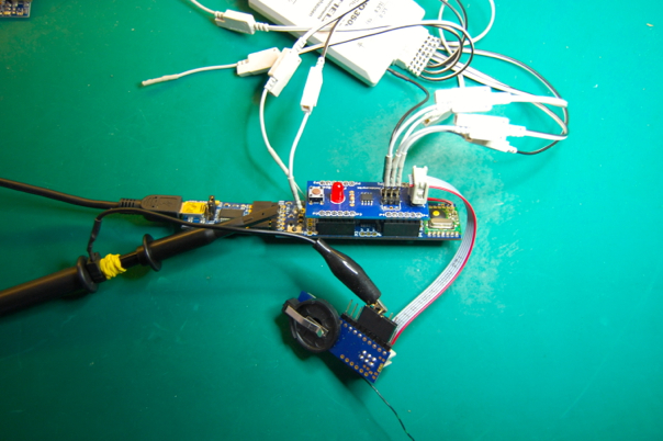
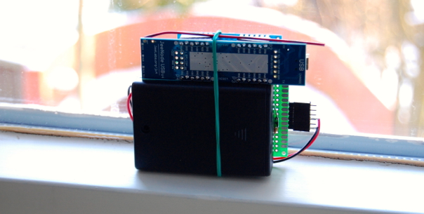
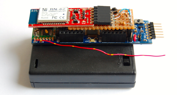
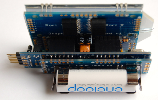
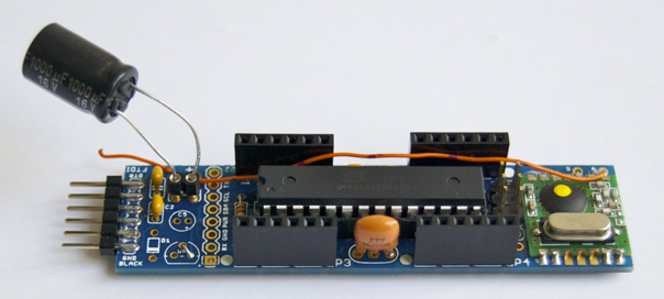
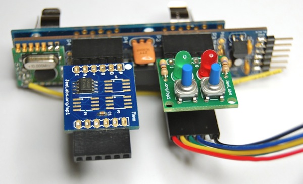
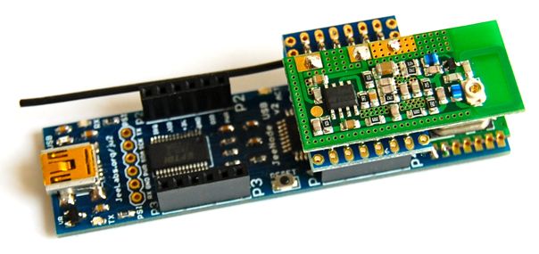
I’m writing this post while one of the test JeeNode Micro’s here at JeeLabs is nearing its eighth month of operation on a single coin cell:

DSC_4507

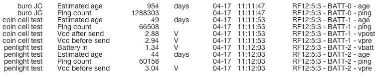
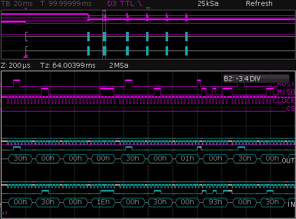
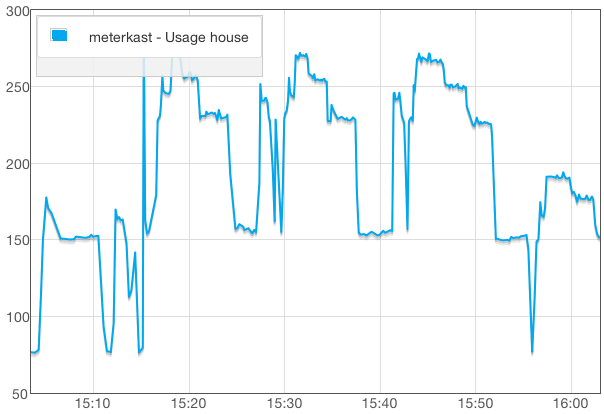
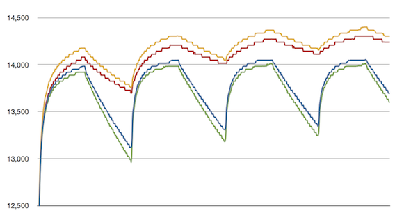
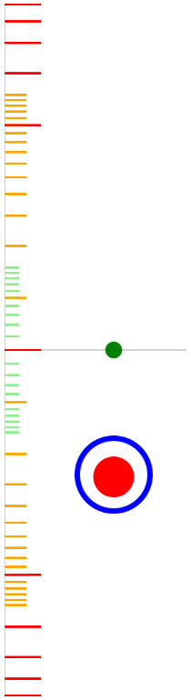
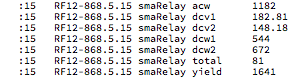
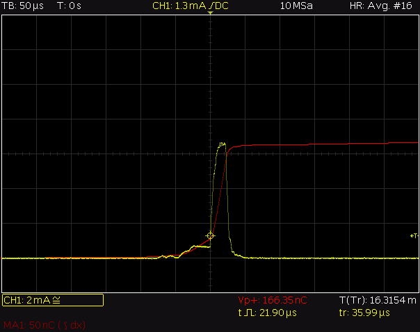
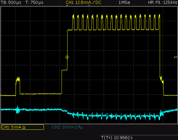
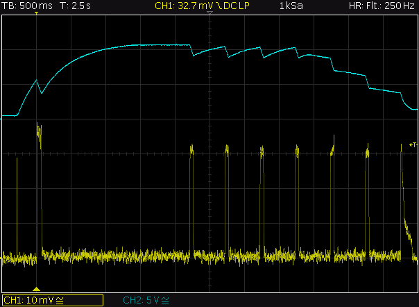
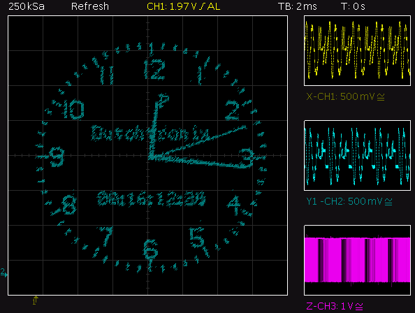
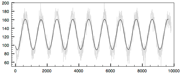
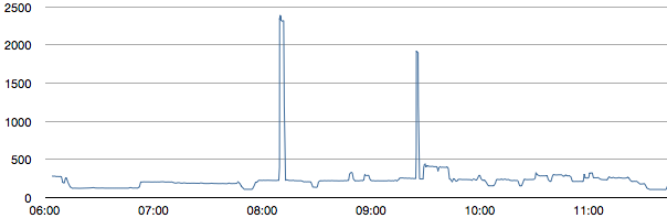
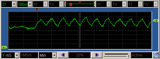
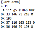
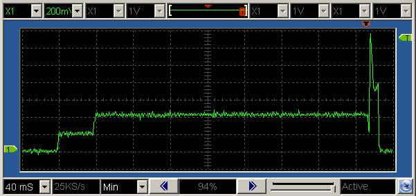
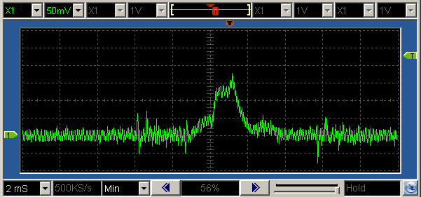
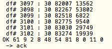
It’s running the radioBlip2 sketch, sending out packets with an incrementing long integer packet count, roughly once every minute:

Screen Shot 2013-10-04 at 15.44.58

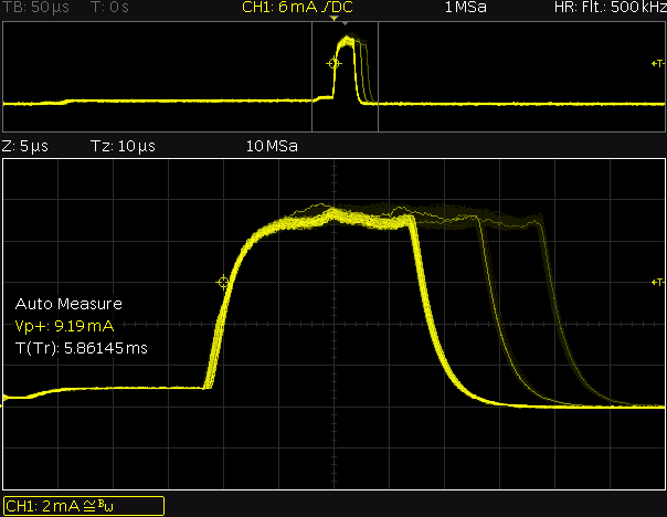
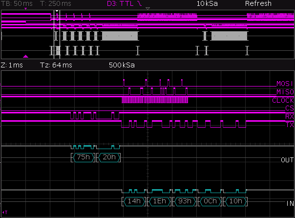
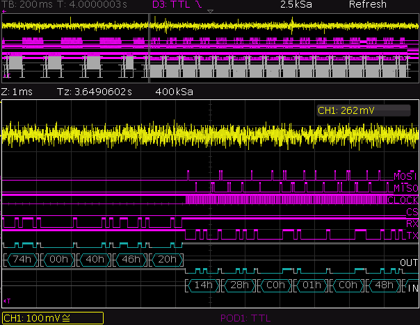
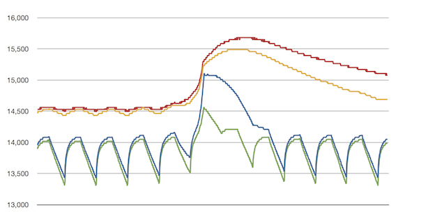
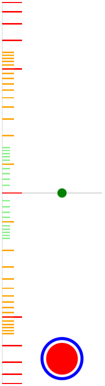
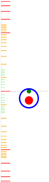
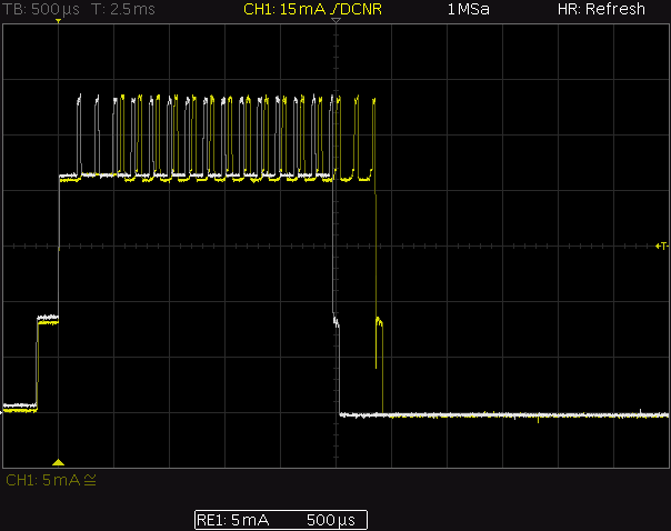
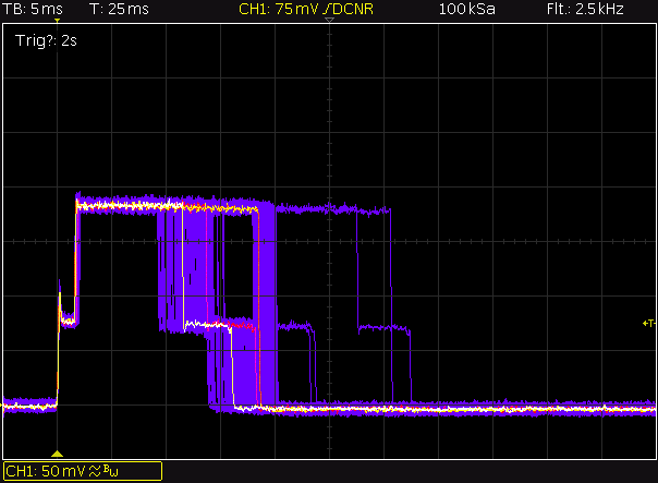
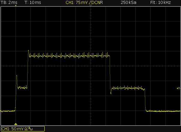
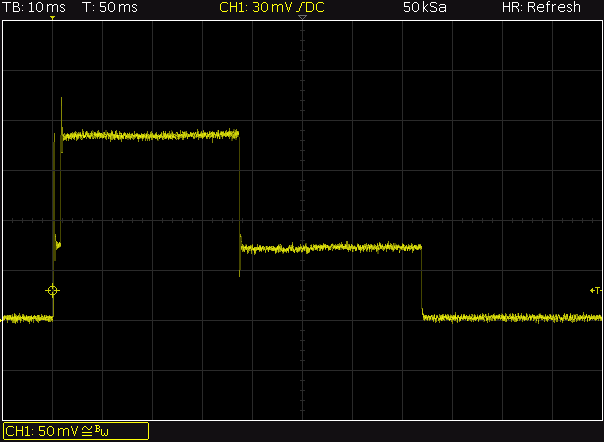
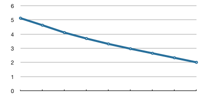
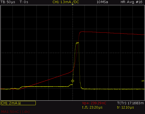
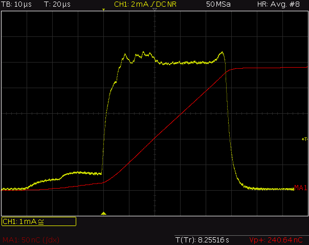
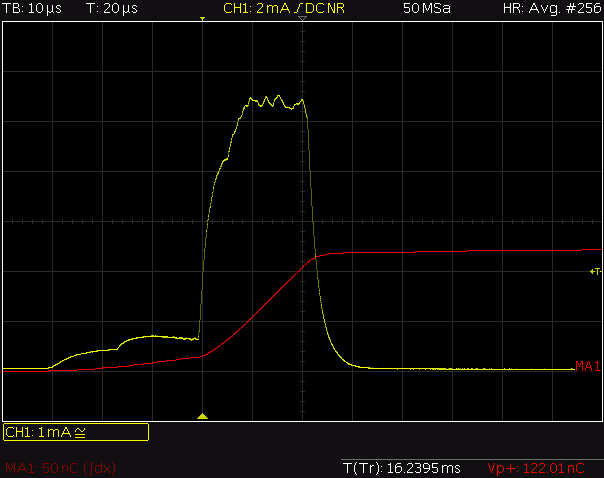
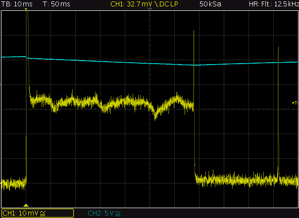
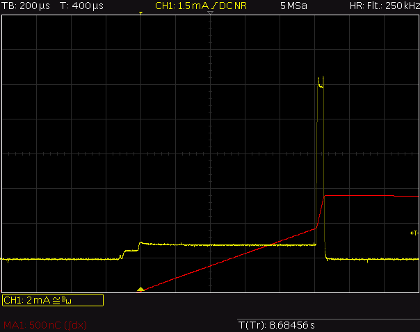
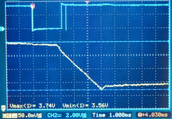
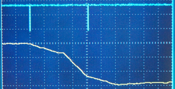
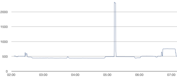
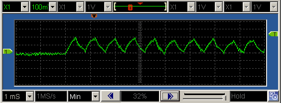
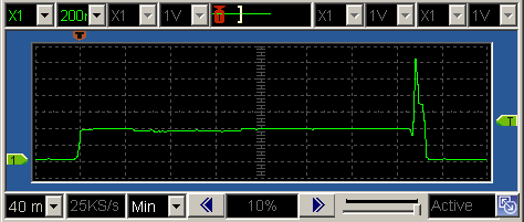
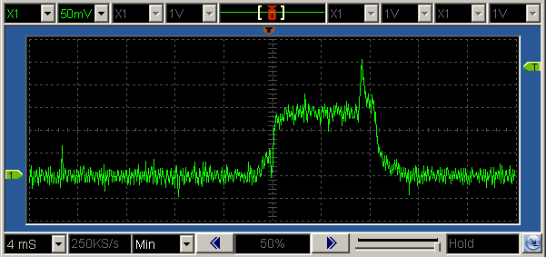
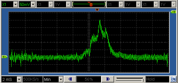
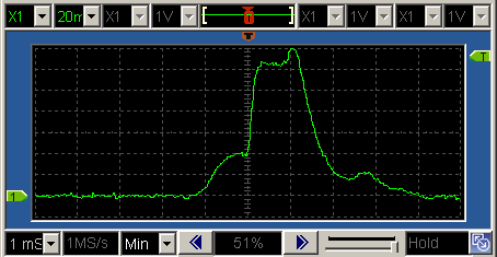
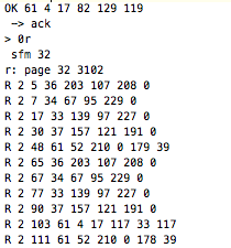
The battery voltage is also tracked, using a nice little trick which lets the ATtiny measure its own supply voltage. As you can see, the battery is getting weaker, dropping in voltage after each 25 mA transmission pulse, but still recovering very nicely before the next transmission:

Screen Shot 2013-10-04 at 15.45.45

Fascinating stuff. A bit like my energy levels, I think :)

But this post is not just about reporting ultra low-power consumption. It’s also my way of announcing that I’ve decided to wrap up this daily weblog and call it quits. There will be no new posts after this one. But this weblog will remain online, and so will the forum & shop.

I know from the many emails I’ve received over the years that many of you have been enjoying this weblog – some of you even from the very beginning, almost 5 years ago. Thank you. Unfortunately, I really need to find a new way to push myself forward.

This is post # 1400, with over 6000 comments to date. Your encouragement, thank-you’s, insightful comments, corrections and additions – I’m deeply grateful for each one of them. I hope that the passion which has always driven me to explore this computing stuff tied to the physical world technology and to write about these adventures, have helped you appreciate the creativity that comes with engineering and invention, and have maybe even tempted you to take steps to explore and learn beyond the things you already knew.

In fact, I sincerely hope that these pages will continue to encourage and inspire new visitors who stumble upon this weblog in the future. For those visitors, here’s a quick summary of the recent flashback posts, to help you find your way around on this weblog:

Please don’t ever stop exploring and pushing the boundaries of imagination and creativity – be it your own or that of others. There is infinite potential in each of us, and I’m certain that if we can tap even just a tiny fraction of it, the world will be a better place.

I’d like to think that I’ve played my part in this and wish you a lot of happy tinkering.

Take care,
Jean-Claude Wippler

PS. For a glimpse of of what I’m considering doing next, see this page. I can assure you that my interests and passions have not changed, and that I’ll remain as active as ever w.r.t. research and product development. The whole point of this change is to allow me to invest more focus and time, and to take the JeeLabs projects and products further, in fact.

PPS. Following the advice of some friends I highly respect, I’m making this last weblog post open-ended: it’ll be the last post for now. Maybe the new plans don’t work out as expected after all, or maybe I’ll want to reconsider after a while, knowing how much joy and energy this weblog has given me over the years. So let’s just call this a break, until further notice :)

Update Dec 2013 – Check out the forum at jeelabs.net for the latest news about JeeLabs.

Flashback – Dive Into JeeNodes

In AVR, Hardware, Software, Linux on Oct 4, 2013 at 00:01

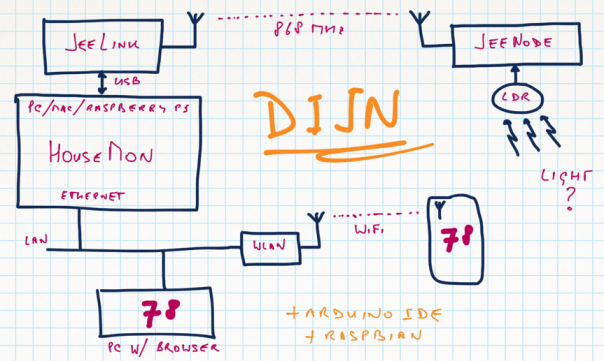
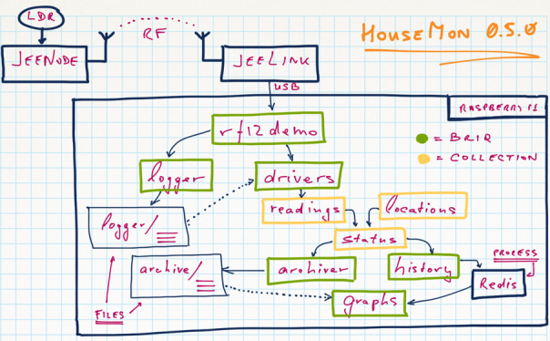
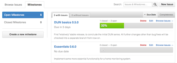
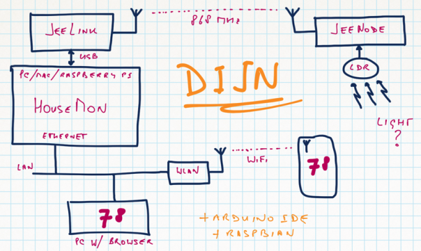
Dive Into JeeNodes (DIJN) is a twelve-part series, describing how to turn one or more remote JeeNodes, a central JeeLink, and a Raspberry Pi into a complete home monitoring setup. Well, ok, not quite: only a first remote setup is described with an LDR as light sensor, but all the steps to make the pieces work together are described.

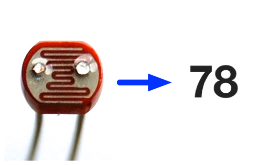
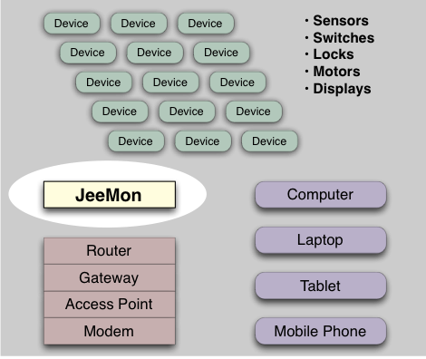
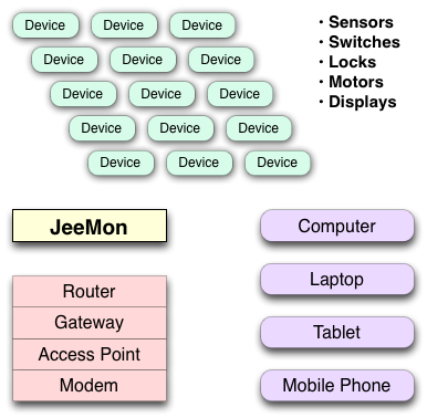
More visually, DIJN describes how to get from here:

dijn01-essence.png   dijn01-diagram

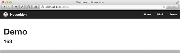
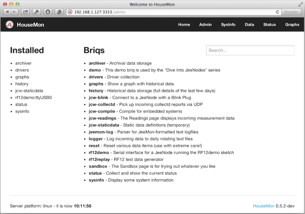
.. to here:

Screen-Shot-2013-02-09-at-12.22.13

This covers a huge range of technologies, from embedded Arduino stuff on an ATmega-based JeeNode, to setting up Node.js and the HouseMon software on a Raspberry Pi embedded Linux board. The total cost of a complete but minimal setup should be around €100. Less than an Xbox and far, far more educational and entertaining, if you ask me!

It’s all about two things really: 1) describing the whole range of technologies and getting things working, and 2) setting up a context which you can explore, learn, and hack on tinker with in numerous ways.

If you’re an experienced Linux developer but want to learn about embedded hardware, wireless sensors, physical computing and such, then this offers a way to hook up all sorts of things on the JeeNode / Arduino side of things.

If you’re familiar with hardware development or have some experience with the Arduino world, then this same setup lets you get familiar with setting up a self-contained low-power Linux server and try out the command line, and many shell commands and programming languages available on Linux.

If you’ve set up a home automation system for yourself in the past, with PHP as web server and MySQL as back end, then this same setup will give you an opportunity to try out rich client-side internet application development based on AngularJS and Node.js – or perhaps simply hook things together so you can take advantage of both approaches.

With the Dive Into JeeNode series, I wanted to single out a specific range of technologies as an example of what can be accomplished today with open source hardware and software, while still covering a huge range of the technology spectrum – from C/C++ running on a chip to fairly advanced client / server programming using JavaScript, HTML, and CSS (or actually: dialects of these, called CoffeeScript, Jade, and Stylus, respectively).

Note that this is all meant to be altered and ripped apart – it’s only a starting point!

Flashback – Ports and I2C in JeeLib

In AVR, Software on Oct 2, 2013 at 00:01

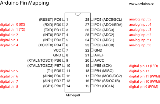
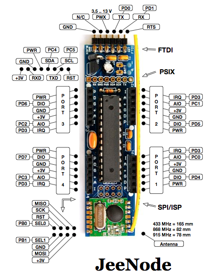
One of the small innovations in the JeeNode is the use of “Ports”:

ports

Most µC boards, including the Arduino, brought out all the I/O pins on one or more large headers, meaning that you had to pick and route individual pins for each case where some component or sensor was being connected. While flexible, it prevented adding stuff in a plug-an-play manner: hook up some sensors, use matching bits of C/C++ code, and done.

I also always kept running out of VCC and GND connection pins while experimenting. So instead of bundling all I/O pins, a decision was made in 2009 to bring out a couple of (nearly) identical “ports”, to any of which the same sensor could be attached. That meant you could connect up to at least four sensors independent of each other.

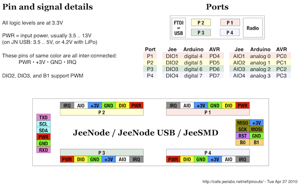
As it turns out, there are enough spare I/O pins on an ATmega to provide one digital and one analog pin to each port. Add GND, VCC (+3.3V) and PWR (the input voltage, could be up to about 13V), and you end up with a fairly general-purpose setup. One extra spare pin was provided as “IRQ” to allow connected sensors to draw attention to themselves via an interrupt, although this feature has admittedly so far not been used much on JeeNodes.

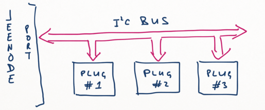
But the real improvement is the fact that the two I/O pins can be used as I2C bus. All of a sudden, each port is no longer limited to a single sensor. The I2C bus is so useful because many types of low-cost chips include an I2C interface in hardware, and it lets multiple chips operate on a single bus.

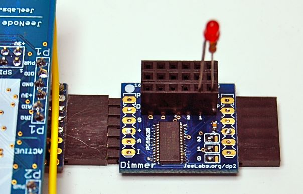
One of the first extensions added was the Expander Plug, an 8-bit general-purpose digital I/O interface. So now, with just two pins consumed on the ATmega, you could have up to 32 input/output pins (by daisy chaining 4 of these plugs and setting them each to a different I2C address). The Dimmer Plug takes this even further: up to 8 of them on one bus, each driving up to 16 LED’s – for a total of 128 dimmable LEDs on 2 I/O pins!

Officially, the I2C bus requires dedicated hardware with “slew control” to increase the accuracy of signals on the bus. And while the ATmega has such an interface, there is just one per ATmega. Fortunately, you can also “bit-bang” I2C in plain software, i.e. simulate the relatively slow pin changes with nothing but software on any 2 I/O pins. The speed is not quite as high, and the supported bus length is also limited to a few dozen centimeters, but for direct connection of a few plugs that still works out quite well.

And so the JeeNode has ended up having 4 “ports”, each of them individually capable of supporting either I2C, or one analog (AIO) and one digital (DIO) pin – or alternately 2 digital I/O’s, since each analog pin on the ATmega can also be used in digital mode.

Since then, lots of different types of “JeePlugs” have been created, some I2C, some not. Most of the plugs have a corresponding class and a demo sketch in the JeeLib library, making it very easy to hook them up and interface to them in software. With most plugs, you just have to define which port they are connected to – and in the case of I2C plugs, which bus address they have been set to.

The placement of these ports and the choice of very low-cost standard 6-pin headers took some experimentation, but I think it all turned out ok. Lots of expandability and flexibility.

Flashback – Batteries came later

In AVR, Hardware, Software on Sep 30, 2013 at 00:01

During all this early experimentation in 2008 and 2009, I quickly zoomed in on the little ATmega + RFM12B combo as a way to collect data around the house. But I completely ignored the power issue…

The necessity to run on battery power was something I had completely missed in the beginning. Everyone was running Arduino’s off either a 5V USB adapter or – occasionally – off a battery pack, and never much more than a few days. Being “untethered” in many projects at that time, meant being able to do something for a few hours or a day, and swapping or recharging batteries at night was easy, right?

It took me a full year to realise that a wireless “node” tied to a wire to run for an extended period of time made no sense. Untethered operation also implies being self-powered:

DSC_0496

Evidently, having lots of nodes around the house would not work if batteries had to be swapped every few weeks. So far, I just worked off the premise that these nodes needed to be plugged into a power adapter – but there are plenty of cases where that is extremely cumbersome. Not only do you need a power outlet nearby, you need fat power adapters, and you have to claim all those power outlets for permanent use. It really didn’t add up, in terms of cost, and especially since the data was already being exchanged wirelessly!

Thus started the long and fascinating journey of trying to run a JeeNode on as little power as possible – something most people probably know this weblog best for. Over the years, it led to some new (for me) insights, such as: transmission draws a “huge” 25 mA, but it’s still negligible because the duration is only a few milliseconds. By far the most important parameter to optimise for is sleep-mode power consumption of the entire circuit.

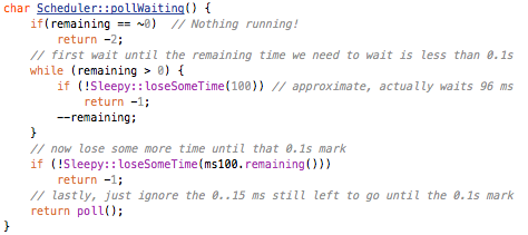
In September 2010, i.e. one year after starting on this low-power journey, the Sleepy class was added to JeeLib, as a way to make it easy to enter low-power mode:

class Sleepy {
public:
    /// start the watchdog timer (or disable it if mode < 0)
    /// @param mode Enable watchdog trigger after "16 << mode" milliseconds 
    ///             (mode 0..9), or disable it (mode < 0).
    static void watchdogInterrupts (char mode);
    
    /// enter low-power mode, wake up with watchdog, INT0/1, or pin-change
    static void powerDown ();
    
    /// Spend some time in low-power mode, the timing is only approximate.
    /// @param msecs Number of milliseconds to sleep, in range 0..65535.
    /// @returns 1 if all went normally, or 0 if some other interrupt occurred
    static byte loseSomeTime (word msecs);

    /// This must be called from your watchdog interrupt code.
    static void watchdogEvent();
};

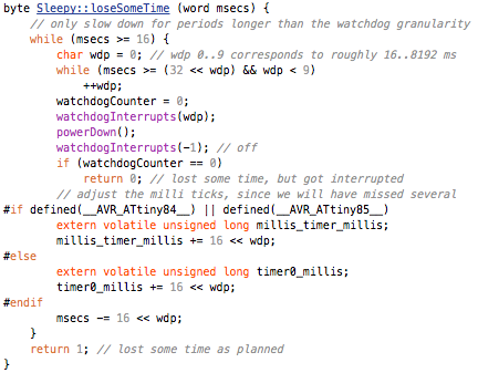
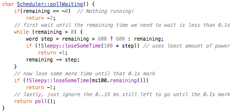
The main call was named loseSomeTime() to reflect the fact that the watchdog timer is not very accurate. Calling Sleepy::loseSomeTime(60000) gives you approximately one minute of ultra low-power sleep time, but it could be a few seconds more or less. To wait longer, you can call this code a few times, since 65,535 ms is the maximum value supported by the Sleepy class.

As a result of this little class, you can do things like put the RFM12B into sleep mode (and any other power-hungry peripherals you might have connected), go to sleep for a bit, and restore all the peripherals to their normal state. The effects can be quite dramatic, with a few orders of magnitude less power consumption. This extends a node’s battery lifetime from a few days to a few years – although you have to get all the details right to get there.

One important design decision in the JeeNode was to use a voltage regulator with a very low idle current (the MCP1700 draws 2 µA idle). As a result, when a JeeNode goes to sleep, it can be made to draw well under 10 µA.

Most nodes here at JeeLabs now keep on running for well over a year on a single battery charge. Everything has become more-or-less install and forget – very convenient!

Flashback – RFM12B wireless

In AVR, Hardware, Software on Sep 29, 2013 at 00:01

After the ATmega µC, the second fascinating discovery in 2008 was the availability of very low-cost wireless modules, powerful enough to get some information across the house:

wireless-modules

It would take another few months until I settled on the RFM12B wireless module by HopeRF, but the uses were quickly falling into place – I had always wanted to track the energy consumption in the house, to try and identify the main energy consumers. That knowledge might then help reduce our yearly energy consumption – either by making changes to the house, or – as it turned out – by simply adjusting our behaviour a bit.

Here is the mouse trap which collected energy metering data at JeeLabs for several years:

mousetrap

This is also when I found Modern Devices’s Real Bare Bone Board Arduino clone by Paul Badger – all the good stuff of an Arduino, without the per-board FTDI interface, and with a much smaller form factor.

Yet another month would pass to get a decent interrupt-driven driver working, and some more tweaks to make transmission interrupt-based as well. The advantage of such as design is that you get the benefits of a multi-tasking setup without all the overhead: the RF12 driver does all its time-critical work in the background, while the main loop() can continue to use delay() calls and blocking I/O (including serial port transmission).

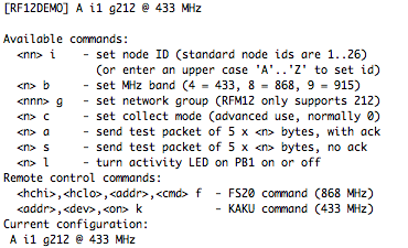
In February 2009, I started installing the RF12demo code on each ATmega, as a quick way to test and try out wireless. As it turned out, that sketch has become quite useful as central receiving node, even “in production” – and I still use it as interface for HouseMon.

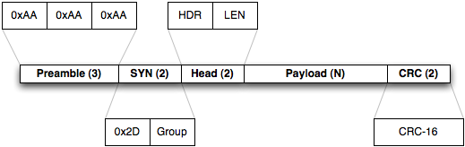
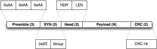
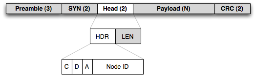
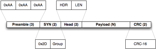
In April 2009, a small but important change was made to the packet format, allowing more robust use of multiple netgroups. Without this change, a bit error in the netgroup byte will alter the packet in a way which is not caught by the CRC checksum, making it a valid packet in another netgroup. This is no big deal if you only use a single netgroup, but will make a difference when multiple netgroups are in use in the same area.

Apart from this change, the RF12 driver and the RFM12B modules have been remarkably reliable, with many nodes here communicating for years on end without a single hick-up.

I still find it pretty amazing that simple low-power wireless networking is available at such a low cost, with very limited software involvement, and suitable for so many low-speed data collection and signalling uses in and around the house. To me, wireless continues to feel like magic after all these years: things happening instantly and invisibly across a distance, using physical properties which we cannot sense or detect…

LevelDB, MQTT, and Redis

In Software on Sep 27, 2013 at 00:01

To follow up on yesterday’s post, here are some more interesting properties of LevelDB, in the context of Node.js and HouseMon:

  • The levelup wrapper for Node supports streaming, i.e. traversing a set of entries for reading, as well as sending an entire set of PUTs and/or DELs as a stream of requests. This is a very nice match for Node.js and for interfaces which need to be sent across the network (including to/from browsers).

  • Events are generated for each change to the database. These can easily be translated into a “live stream” of changes. This is really nothing other than publish / subscribe, but again in a form which matches Node’s asynchronous design really well.

  • Standard encoding conventions can be defined for keys and or values. In the case of HouseMon, I’m using UTF-8 as key encoding default and JSON as value encoding. The latter means that the default “stuff” stored in the database is simply a JavaScript object, and this is also what you get back on access and traversal. Individual cases can still override these defaults.

Together, all these features and conventions end up playing together very nicely. One particularly interesting aspect is the “persistent pub-sub” model you can implement with this. This is an area where the “Message Queue Telemetry Transport” MQTT has been gaining a lot of attention for things like home automation and the “Internet of Things” IoT.

MQTT is a message-based system. There are channels, named in a hierarchical manner, e.g. “/location/device/sensor”, to which one can publish measurement values (“publish /kitchen/roomnode/temp 17”). Other devices or software can subscribe to such channels, and get notified each time a value is published.

One interesting aspect of MQTT is its “RETAIN” functionality: for each channel, the last value can be retained, meaning that anyone subscribing to a channel will immediately be sent the last retained value, as if it just happened. This turns an ephemeral message-based setup into a state-based mechanism with change propagation, because you can subscribe to a channel after devices have published new values on it, yet still see what the best known value for that channel is, currently. With RETAIN, the MQTT system becomes a little database, with one value per channel. This can be very convenient after power-up as well.

LevelDB comes from the other side, i.e. a database with change tracking, but the effect is exactly the same: you can subscribe to a set of keys, get all their latest values and be notified from that point on whenever any keys in this range changes. This makes LevelDB and MQTT functionally equivalent, although LevelDB can handle much larger key spaces (note also that MQTT has features which LevelDB lacks, such as QoS).

It’s also interesting to compare this with the Redis database: Redis is another key-value store, but with more data structure options. The main difference with LevelDB, is that Redis is memory-based, with periodic snapshots to disk, whereas LevelDB is disk based, with caching in memory (and thus able to handle datasets which far exceed available RAM). Redis, LevelDB, and MQTT all support pub-sub in some form.

One reason for me to select LevelDB for HouseMon, is that it’s an in-process embedded database. This means that there is no need for a separate process to run alongside Node.js – and hence to need to install anything, or keep a background daemon running.

By switching to LevelDB, the HouseMon installation procedure has been simplified to:

  • download a recent version of HouseMon from GitHub
  • install Node (which includes the “npm” package manager)
  • run “npm install” to get everything needed by HouseMon

And that’s it. At this point, you just start up Node.js and everything will work.

But it’s not just convenience. LevelDB is also so compact, performant, and scalable, that HouseMon can now store all raw data as well as a complete set of aggregated per-hour values without running into resource limits, even on a Raspberry Pi. According to my rough estimates, it should all end up using less than 1 GB per year, so everything will easily fit on an 8 or 16 GB SD card.

The LevelDB database

In Software on Sep 26, 2013 at 00:01

In recent posts, I’ve mentioned LevelDB a few times – a database with some quite interesting properties.

Conceptually, LevelDB is ridiculously simple: a “key-value” store which stores all entries in sorted key order. Keys and values can be anything (including empty). LevelDB is not a toy database: it can handle hundreds of millions of keys, and does so very efficiently.

It’s completely up to the application how to use this storage scheme, and how to define key structure and sub-keys. I’m using a simple prefix-based mechanism: some name, a “~” character, and the rest of the key, of which each field can be separated with more “~” characters. The implicit sorting then makes it easy to get all the keys for any prefix.

LevelDB is good at only a few things, but these work together quite effectively:

  • fast traversal in sorted and reverse-sorted order, over any range of keys
  • fast writing, regardless of which keys are being written, for add / replace / delete
  • compact key storage, by compressing common prefix bytes
  • compact data storage, by a periodic compaction using a fast compression algorithm
  • modifications can be batched, with a guaranteed all-or-nothing success on completion
  • traversal is done in an isolated manner, i.e. freezing the state w.r.t. further changes

Note that there are essentially just a few operations: GET, PUT, DEL, BATCH (of PUTs and DELs), and forward/backward traversal.

Perhaps the most limiting property of LevelDB is that it’s an in-process embedded library, and that therefore only a single process can have the database open. This is not a multi-user or multi-process solution, although one could be created on top by adding a server interface to it. This is the same as for Redis, which runs as one separate process.

To give you a rough idea of how the underlying log-structured merge-tree algorithm works, assume you have a datafile with a sorted set of key-value pairs, written sequentially to file. In the case of LevelDB, these files are normally capped at 2 MB each, so there may be a number of files which together constitute the entire dataset.

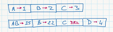
Here’s a trivial example with three key-value pairs:

one-level

It’s easy to see that one can do fast read traversals either way in this data, by locating the start and end position (e.g. via binary search).

The writing part is where things become interesting. Instead of modifying the files, we collect changes in memory for a bit, and then write a second-level file with changes – again sorted, but now not only containing the PUTs but also the DELs, i.e. indicators to ignore the previous entries with the same keys.

Here’s the same example, but with two new keys, one replacement, and one deletion:

two-levels

A full traversal would return the entries with keys A, AB, B, and D in this last example.

Together, these two levels of data constitute the new state of the database. Traversal now has to keep track of two cursors, moving through each level at the appropriate rate.

For more changes, we can add yet another level, but evidently things will degrade quickly if we keep doing this. Old data would never get dropped, and the number of levels would rapidly grow. The cleverness comes from the occasional merge steps inserted by LevelDB: once in a while, it takes two levels, runs through all entries in both of them, and produces a new merged level to replace those two levels. This cleans up all the obsolete and duplicate entries, while still keeping everything in sorted order.

The consequence of this process, is that most of the data will end up getting copied, a few times even. It’s very much like a generational garbage collector with from- and to-spaces. So there’s a trade-off in the amount of writing this leads to. But there is also a compression mechanism involved, which reduces the file sizes, especially when there is a lot of repetition across neighbouring key-value pairs.

So why would this be a good match for HouseMon and time series data in general?

Well, first of all, in terms of I/O this is extremely efficient for time-series data collection: a bunch of values with different keys and a timestamp, getting inserted all over the place. With traditional round-robin storage and slots, you end up touching each file in some spot all the time – this leads to a few bytes written in a block, and requires a full block read-modify-write cycle for every single change. With the LevelDB aproach, all the changes will be written sequentially, with the merge process delayed (and batched!) to a different moment in time. I’m quite certain that storage of large amounts of real-time measurement data will scale substantially better this way than any traditional RRDB, while producing the same end results for access. The same argument applies to indexed B-Trees.

The second reason, is that data sorted on key and time is bound to be highly compressible: temperature, light levels, etc – they all tend to vary slowly in time. Even a fairly crude compression algorithm will work well when readings are laid out in that particular order.

And thirdly: when the keys have the time stamp at the end, we end up with the data laid out in an optimal way for graphing: any graph series will be a consecutive set of entries in the database, and that’s where LevelDB’s traversal works at its best. This will be the case for raw as well as aggregated data.

One drawback could be the delayed writing. This is the same issue with Redis, which only saves its data to file once in a while. But this is no big deal in HouseMon, since all the raw data is being appended to plain-text log files anyway – so on startup, all we have to do is replay the end of the last log file, to make sure everything ends up in LevelDB as well.

Stay tuned for a few other reasons on why LevelDB works well in Node.js …

In search of a good graph

In Software on Sep 24, 2013 at 00:01

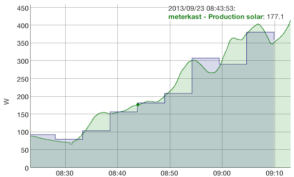
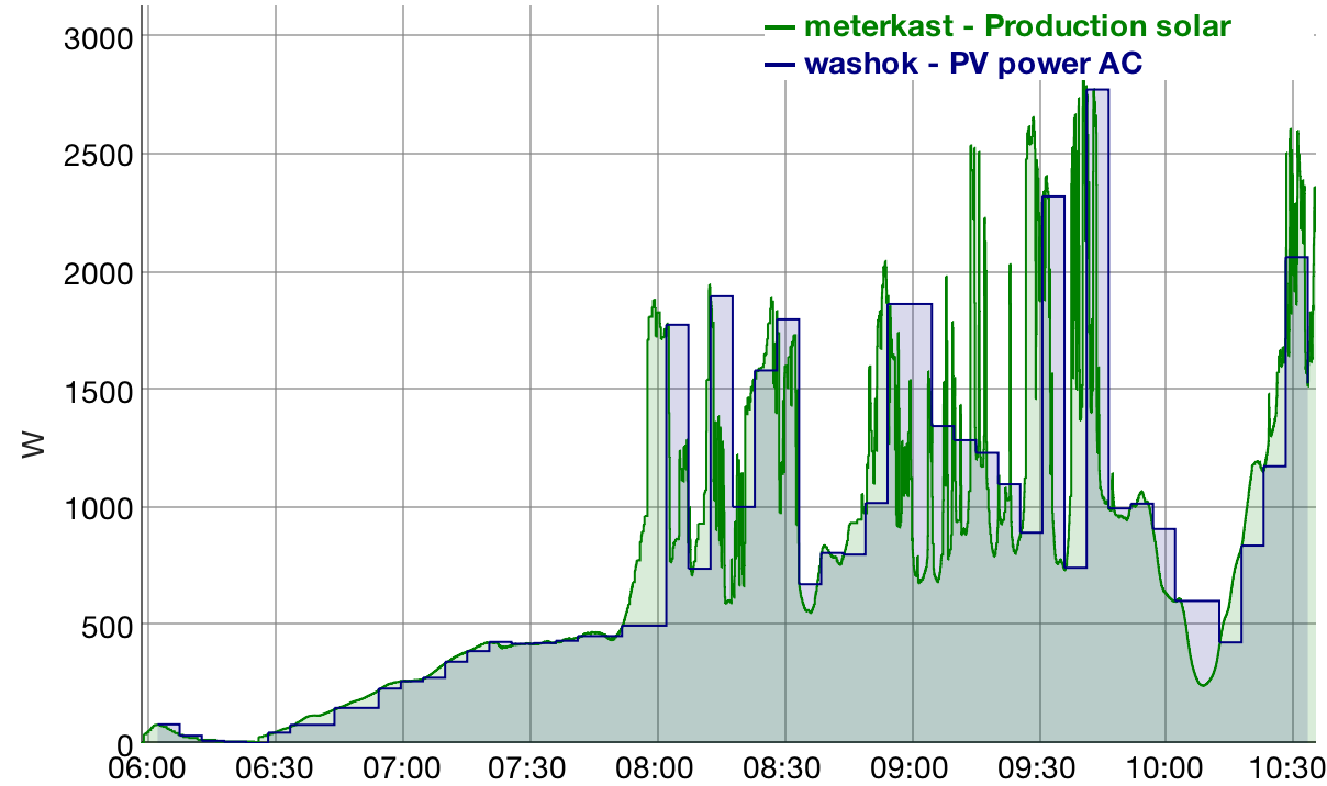
I’ve been using the DyGraphs package for some time now in HouseMon, but it’s not perfect. Here is a generated graph for this morning, comparing two different ways to measure the same solar power generation:

Screen Shot 2013-09-23 at 09.20.52

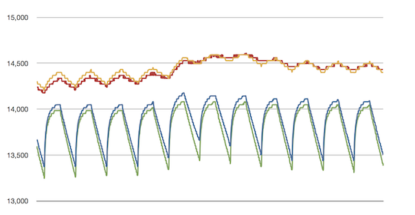
The green series comes from the a pulse counter which generates a pulse every 0.5 Wh. These values then get sent to HouseMon every 3 seconds. A fairly detailed set of readings, as you can see – this is a typical morning in autumn on a cloudy day.

The blue series comes from the SMA inverter, which I’m reading every 5..6 minutes. It might be more accurate, but there is far less data coming in.

The key is that the area (i.e. Wh) under these two lines should be identical, if both devices are accurately calibrated. But this doesn’t quite seem to be the case here. (see update)

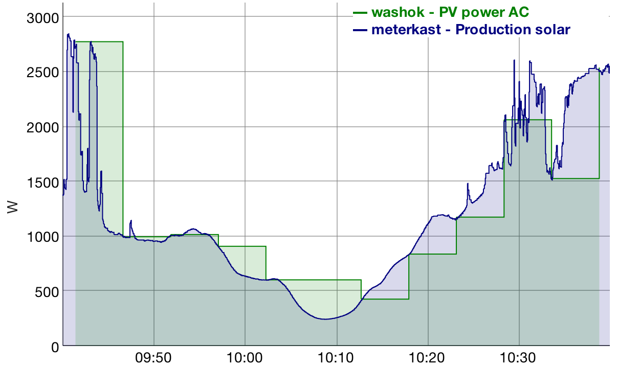
One known problem is that DyGraphs is plotting these “step charts” incorrectly: the value of the step should be at the end of the step, but DyGraphs can only plot steps given a starting value. So the way to read these blue steps, I think, is to keep the points, but to think of the step lines as being drawn horizontally preceding that point, not trailing it. I’m not fully convinced that this explains all the differences in the above examples, but it would seem to be a better match.

I’ve been looking at Highcharts and Highstocks as an alternative graphing library to use. They seem to support steps-with-end-values. But this sort of use really has quite a few other requirements as well, such as: being able to draw large datasets efficiently, support for multiple independent time series (DyGraphs was a bit limited here as well), interactive and intuitive zooming, good automatic choice of axis scales and fonts.

It would also be nice to be able to efficiently redraw a graph when new data points come in. Graphs used to be live in HouseMon, but at some point I ran into a snag and never bothered to fix it. For me, right now, live updating is less important than being able to generate accurate graphs. What’s the point of showing results on screen after all, if those results are not really represented truthfully…

I’ll stay on the lookout for better graphing solution. All suggestions welcome!

Update – See @ward’s comments below for the proper explanation of what’s going on here. It’s not a graphing problem after all (or rather: a different one…).

Animation in the browser

In Software on Sep 23, 2013 at 00:01

If you’ve programmed for Mac OS X (my actual experience in that area is fairly minimal), then you may know that it has a feature called Core Animation – as a way to implement all sorts of flashy smooth UI transitions – sliding, fading, colour changes, etc.

The basic idea of animation in this context is quite simple: go from state A to state B by varying one or more values gradually over a specified amount of time.

It looks like web browsers are latching onto this trend as well, with CSS Animations. It has been possible to implement all sorts of animations for some time, using timed JavaScript loops running in the background to simulation this sort of stuff, as jQuery has been doing. Then again, getting such flashy features into a whole set of independently-developed (and competing) web browsers is bound to take more time, but yeah… it’s happening. Here’s an illustration of what text can do in today’s browsers.

In Angular, browser-side animation has recently become quite a bit simpler.

I’m no big fan of attention-drawing screen effects. There was a time when HTML’s BLINK tag got so much, ehm, attention that every page tried to look like a neon sign. Oh, look, a new toy tag, and it’s BLINKING… neat, let’s use it everywhere!

Even slide transitions (will!) get boring after a while.

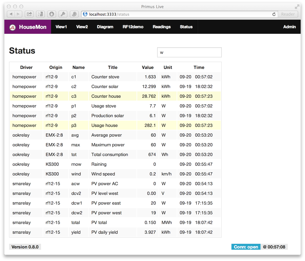
But with dynamic web pages updating in real time, it seems to me that there is a case to be made for subtle hints that something has just happened. As trial, I used a fade transition (from jQuery) in the previous version of HouseMon to briefly change the background of a changed row to very light yellow, which then fades back to white:

Screen Shot 2013-09-22 at 20.26.32

The effect seems to work well – for me anyway: it’s easy to spot the latest changes in a table, without getting too distracted when looking at some specific data.

In the latest version of HouseMon, I wanted to try the same effect using the new Angular animation feature, and I must say: the basic mechanism is really simple – you make animations happen by defining the CSS start settings, the finish settings, and the time period plus transition style to use. In the case of adding a row to a table or deleting a row, it’s all built-in and done by just adding some CSS definitions, as described here.

In this particular case, things are slightly more involved because it’s not the addition or deletion of a row I wanted to animate, but the change of a timestamp on a row. This requires defining a custom Angular “directive”. Directives are the cornerstone of Angular: they can (re-) define the behaviour of HTML elements or attributes, and let you invent new ones to do just about anything possible in the DOM.

Unfortunately, directives can also be a bit obscure at times. Here is the one I ended up defining for HouseMon:

ng.directive 'highlightOnChange', ($animate) ->                                  
  (scope, elem, attrs) ->                                                        
    scope.$watch attrs.highlightOnChange, ->                                     
      $animate.addClass elem, 'highlight', ->                                    
        attrs.$removeClass 'highlight'   

With it, we can now use a new custom highlightOnChange attribute to an element to implement highlighting when a value on the page changes.

Here is how it gets used (in Jade) on the status table rows shown in yesterday’s post:

tr(highlight-on-change='row.time')

In prose: when row.time changes, start the highlight transition, which adds a custom highlight class and removes it again at the end of the animation sequence.

The CSS then defines the actual animation (using Stylus notation):

.highlight-add
  transition 1s linear all
  background lighten(yellow, 75%)
.highlight-add.highlight-add-active
  background white

I’m leaving out some finicky details, but that’s the essence of it all: set up an $animate call to trigger on the proper conditions, and then define what is going go happen in CSS.

Note that Angular picks name suffixes for the CSS classes during the different phases of animation, but then it can all be used for numerous types of animation: you pick the CSS setting(s) at start and finish, and the browser’s CSS engine will automatically “run” the selected animation – covering motions, colour changes, and lots more (could fonts be emboldened gradually or even be morphed in more sophisticated ways? I haven’t tried it).

The result of all this is a table with subtle row highlights wherever a new reading comes in. Triggered by some Angular magic, but the actual highlighting is a (not-yet-100%-standardised) browser effect.

Working with a CSS grid

In Software on Sep 22, 2013 at 00:01

As promised yesterday, here is some information on how you can get a page layouts off the ground real quick with the Zurb Foundation 4 CSS framework. If you’re more into Twitter Bootstrap, see this excellent comparison and overview. They are very similar.

It took a little while to sink in, until I read this article about how it’s supposed to be used, and skimmed through a 10-part series on webdesign tuts+. Then the coin dropped:

  • you create rows of content, using a div with class row
  • each row has 12 columns to put stuff in
  • you put the sections of your page content in divs with class large-6 and columns
  • each section goes next to the preceding one, so 6 and 6 puts the split in the middle
  • any number from 1 to 12 goes, as long as you use at most 12 columns per row

So far so good, and pretty trivial. But here’s where it gets interesting:

  • each column can have more rows, and each row again offers 12 columns to lay out
  • for mobile use, you can add small-N classes as well, with other column allocations

I haven’t done much with this yet, but this page was trivial to generate:

Screen Shot 2013-09-20 at 00.57.16

The complete definition of that inner layout is in app/status/view.jade:

.row
  .large-9.columns
    .row
      .large-8.columns
        h3 Status
      .large-4.columns
        h3
        input(type='text',ng-model='statusQuery',placeholder='Search...')
    .row
      .large-12.columns
        table(width='100%')
          tr
            th Driver
            th Origin
            th Name
            th Title
            th Value
            th Unit
            th Time
          tr(ng-repeat='row in status | filter:statusQuery | orderBy:"key"')
            td {{row.type}}
            td {{row.tag}}
            td {{row.name}}
            td {{row.title}}
            td(align='right') {{row.value}}
            td {{row.unit}}
            td {{row.time | date:"MM-dd &nbsp; HH:mm:ss"}}

In prose:

  • the information shown uses the first 9 columns, (the remaining 3 are unused)
  • in those 9 columns, we have a header row and then the actual data table as row
  • the header is a h1 header on the left and an input on the right, split as 2:1
  • the table takes the full width (of those 9 columns in which it resides)
  • the rest is standard HTML in Jade notation, and an Angular ng-repeat loop
  • there’s also live row filtering in there, using some Angular conventions
  • the alternating row backgrounds and general table style are Foundation’s defaults

Actually, I left out one thing: the entries automatically get highlighted whenever the time stamp changes. This animation is a nice way to draw attention to updates – stay tuned.

Responsive CSS layouts

In Software on Sep 21, 2013 at 00:01

One of the things today’s web adds to the mix, is the need to address devices with widely varying screen sizes. Seeing a web site made for an “old” 1024×768 screen layout squished onto a mobile phone screen is not really great if everything just ends up smaller on-screen.

Enter grid-based CSS frameworks and responsive CSS.

There’s a nice site to quickly try designs at different sizes, at cybercrab.com/screencheck. Here’s how my current HouseMon screen looks on two different simulated screens:

Screen Shot 2013-09-19 at 23.45.02

Screen Shot 2013-09-20 at 00.17.54

It’s not just reflowing CSS elements (the bottom line stacks vertically on a small screen), it also completely alters the behaviour of the navigation bar at the top. In a way which works well on small screens: click in the top right corner to fold out the different menu choices.

Both Zurb Foundation and Twitter Bootstrap are “CSS frameworks” which provide a huge set of professionally designed UI elements – and now also do this responsive thing.

The key point here is that you don’t need to do much to get all this for free. It takes some fiddling and googling to set all the HTML sections up just right, but that’s it. In my case, I’m using Angular’s “ng-repeat” to generate the navigation bar menu entries on-the-fly:

nav.top-bar(ng-controller='NavCtrl')
  ul.title-area
    li.name
      h1
        a(ng-href='{{appInfo.home}}')
          img(src='/main/logo.png',height=22,width=22)
          | &nbsp; {{appInfo.name}}
    li.toggle-topbar.menu-icon
      a(href='#')
        span
  section.top-bar-section
    ul.left
      li.myNav(ng-repeat='nav in navbar')
        a(ng-href='{{nav.route}}') {{nav.title}}
      li.divider
    ul.right
      li.myNav
        a(href='/admin') Admin

Yeah, ok, pretty tricky stuff. But it’s all documented, and nowhere near the effort it’d take to do this sort of thing from scratch. Let alone get the style and visual layout consistent and working across all the different browsers and versions.

Tomorrow, I’ll describe the way grid layouts work with Zurb Foundation 4 – it’s sooo easy!

In praise of AngularJS

In Software on Sep 20, 2013 at 00:01

This is how AngularJS announces itself on its home page:

HTML enhanced for web apps!

Hm, ok, but not terribly informative. Here’s the next paragraph:

HTML is great for declaring static documents, but it falters when we try to use it for declaring dynamic views in web-applications. AngularJS lets you extend HTML vocabulary for your application. The resulting environment is extraordinarily expressive, readable, and quick to develop.

That’s better. Let me try to ease you into this “framework” on which HouseMon is based:

  • Angular (“NG”) is client-side only. It doesn’t exist on the server. It’s all browser stuff.
  • It doesn’t take over. You could use NG for parts of a page. HouseMon is 100% NG.
  • It comes with many concepts, conventions, and terms you must get used to. They rock.

I can think of two main stumbling blocks: “Dependency Injection” and all that “service”, “factory”, and “controller” stuff (not to mention “directives”). And Model-View-Something.

It’s not hard. It wasn’t designed to be hard. The terminology is pretty clever. I’d say that it was invented to produce a mental model which can be used and extended. And like a beautiful clock, it doesn’t start ticking until all the little pieces are positioned just right. Then it will run (and evolve!) forever.

Dependency injection is nothing new, it’s essentially another name for “require” (Node.js), “import” (Python), or “#include” (C/C++). Let’s take a fictional piece of CoffeeScript code:

value = 123
myCode = (foo, bar) -> foo * value + bar

console.log myCode(100, 45)

The output will be “12345”. But with dependency injection, we can do something else:

value = 123
myCode = (foo, bar) -> foo * value + bar

define 'foo', 100
define 'bar', 45
console.log inject(myCode)

This is not working code, but it illustrates how we could define things in some more global context, then call a function and give it access to that context. Note that the “inject” call does something very magical: it looks at the names of myCode’s arguments, and then somehow looks them up and finds the values to pass to myCode.

That’s dependency injection. And Angular uses it all over the place. It will often call functions through a special “injector” and get hold of all args expected by the function. One reason this works is because closures can be used to get local scope information into the function. Note how myCode had access to “value” via a normal JavaScript closure.

In short: dependency injection is a way for functions to import all the pieces they need. This makes them extremely modular (and it’s great for test suites, because you can inject special versions and mock objects to test each piece of code outside its normal context).

The other big hurdle I had to overcome when starting out with Angular, is all those services, providers, factories, controllers, and directives. As it turns out, that too is much simpler than it might seem:

  • Angular code is packaged as “modules” (I actually only use a single one in HouseMon)
  • in these modules, you define services, etc – more on this in a moment
  • the whole startup is orchestrated in a specific way: boot, config, run, fly
  • ok, well, not “fly” – that’s just my name for it…

The startup sequence is key – to understand what goes where, and what gets called when:

  • the browser starts by loading an HTML page with <script> tags in it (doh)
  • all the code needed on the browser side has to be loaded up front
  • what this code does is define modules, services, and so on
  • nothing is really “running” at this point, these are all function definitions
  • the last step is to call angular.bootstrap(document, ['myApp']);
  • at this point, all the config sections defined in the modules are run
  • once that is over, all the run sections are run, this is the real application start
  • when that is done, we in essence enter The Big Event Loop in the browser: lift off!

So on the client side, i.e. the browser, the entire application needs to be structured as a set of definitions. A few things need to be done early on (config), a few more once everything has been defined and Angular’s “$rootScope” has been put in place (read: the main page context is ready, a bit like the DOM’s “document.onload”), and then it all starts doing real work through the controllers tied to various HTML elements in the DOM.

Providers, factories, services, and even constants and values, are merely variations on a theme. There is an excellent page by Matt Haggard describing these differences. It’s all smoke and mirrors, really. Everything except directives is a provider in Angular.

Angular is like the casing of a watch, with a powerful pre-loaded spring already in place. You “just” have to figure out the role of the different pieces, put a few of them in place, and it’ll run all by itself from then on. It’s one of the most elegant frameworks I’ve ever seen.

With HouseMon, I’ve put the main pieces in place to show a web page in the browser with a navigation top bar, and the hooks to tie into Primus and RPC. The rest is all up to the modules, i.e. the subfolders added to the app/ folder. Each client.coffee file is an Angular module. HouseMon will automatically load them all into the browser (via a /primus/primus.js file generated on-the-fly by Primus). This has turned out to be extremely modular and flexible – and it couldn’t have been done without Angular.

If you’re looking for a “way in” for the HouseMon client-side code, then the place to start is app/index.jade, which uses Jade’s extend mechanism to tie into main/layout.jade, so that would be the second place to start. After that, it’s all Angular-structured code, i.e. views, view templates with controllers, and the services they call.

I’m quite excited by all this, because I’ve never before been able to develop software in such a truly modular fashion. The interfaces are high-level, clean (and clear) and all future functionality can now be added, extended, replaced, or even removed again – step by step.

Ground control to… browser

In Software on Sep 19, 2013 at 00:01

After yesterday’s RPC example, which makes the server an easy-to-use service in client code, let’s see how to do things in the other direction.

I should note that there is usually much less reason to do this, since at any point in time there can be zero, one, or occasionally more clients connected to the server in the first place. Still, it could be useful for a server to collect client status info, or to periodically save some state. The benefit of server-initiated requests being that it turns authentication around, assuming we trust the server.

Ok, so here’s some silly code on the client which I’d like to be able to call from the server:

ng = angular.module 'myApp'

ng.config ($stateProvider, navbarProvider, primus) ->
  $stateProvider.state 'view1',
    url: '/'
    templateUrl: 'view1/view.html'
    controller: 'View1Ctrl'
  navbarProvider.add '/', 'View1', 11
  
  primus.client.view1_twice = (x) ->
    2 * x

ng.controller 'View1Ctrl', ->

This is the “View 1” module, similar to the Admin module, exposing code for server use:

  primus.client.view1_twice = (x) ->
    2 * x

On the server side, the first thing to note is that we can’t just call this at any point in time. It’s only available when a client is connected. In fact, if more than one client is connected, then there will be multiple instances of this code. Here is app/view1/host.coffee:

module.exports = (app, plugin) ->
  app.on 'running', (primus) ->
    primus.on 'connection', (spark) ->
      
      spark.client('view1_twice', 123).then (res) ->
        console.log 'double', res

The output on the server console, whenever a client connects, is – rather unsurprisingly:

    double 246

What’s more interesting here, is the logic of that server-side code:

  • the app/view1/host.coffee exports one function, accepting two args
  • when loaded on startup, it will be called with the app and Primus plugin object
  • we’re in setup mode at this point, so this is a good time to define event handlers
  • the app.on 'running' handler gets called when all server setup is complete
  • now we can set up a handler to capture all new client connections
  • when such a connection comes in, Primus will hand us a “spark” to talk to
  • a spark is essentially a WebSocket session, it supports a few calls and streaming
  • now we can call the ‘view1_twice’ code on the client via RPC
  • this creates and returns a promise, since the RPC will take a little bit of time
  • we set it up so that when the promise is fulfilled, console.log ... gets called

And that’s it. As with yesterday’s setup, all the communication and handling of asynchronous callbacks is taken care of behind the scenes.

There is some asymmetry in naming conventions and the uses of promises, but here’s the summary:

  • to define a function ‘foo’ on the host, define it as app.host.foo = …
  • to call that function on the client, use host ‘foo’, …
  • the result is an Angular promise, use “.then …” to pick it up if needed
  • to define a function ‘bar’ on the client, define it as primus.client = …
  • to call that function from the server, use spark.client ‘bar’, …
  • the result is a q promise, use “.then …” to pick it up

Ok, so there are some slight differences between the two promise API’s. But the main benefit of this all is that the passing of time and networking involved is completely abstracted away. Maybe I’ll be able to unify this further, some day.

Promise-based RPC

In Software on Sep 18, 2013 at 00:01

Or maybe this post should have been titled: “Taming asynchronous RPC”.

Programming with asynchronous I/O is tricky. The proper solution IMO, is to have full coroutine or generator support in the browser and in the server. This has been in the works from some time now (see ES6 Harmony). In short: coroutines and generators can “yield”, which means something that takes time can suspend the current stack state until it gets resumed. A bit like green (non-preemptive) threads, and with very little overhead.

But we ain’t there yet, and waiting for all the major browsers to reach that point might be a bit of a stretch (see the “Generators (yield)” entry on this page). The latest Node.js v0.11.7 development release does seem to support it, but that’s only half the story.

So promises it is for now. On the server side, this is available via Kris Kowal’s q package. On the client side AngularJS includes promises as $q. And as mentioned before, I’m also using q-connection as promise-based Remote Procedure Call RPC mechanism.

The result is really neat, IMO. First, RPC from the client, calling a function on the server. This is app/admin/client.coffee for the client side:

ng = angular.module 'myApp'

ng.config ($stateProvider) ->
  $stateProvider.state 'admin',
    url: '/admin'
    templateUrl: 'admin/view.html'
    controller: 'AdminCtrl'

ng.controller 'AdminCtrl', ($scope, host) ->
  $scope.hello = host 'admin_dbinfo'

This Angular boilerplate defines an Admin page with app/admin/view.jade template:

h3 Storage use
table
  tr
    th Group
    th Size
  tr(ng-repeat='(group,size) in hello')
    td {{group}}
    td(align='right') ≈ {{size}} b

The key is this one line:

$scope.hello = host 'admin_dbinfo'

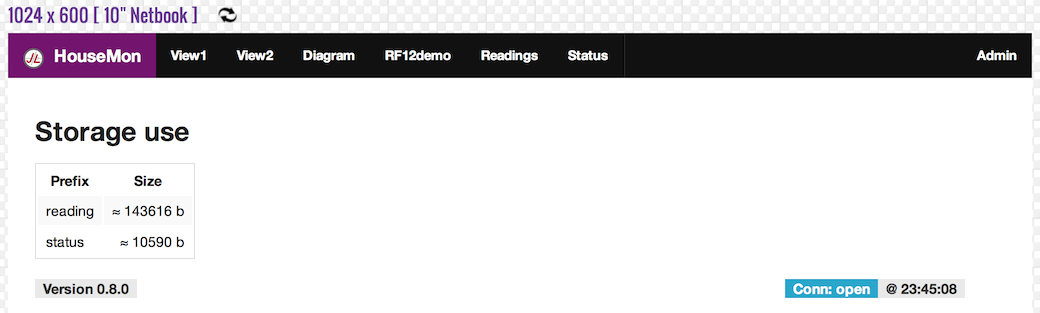
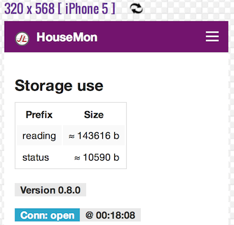
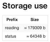
That’s all there is to doing RPC with a round-trip over the network. And here’s the result, as shown in the browser (formatted with the Zurb Foundation CSS framework):

Screen Shot 2013-09-17 at 13.37.33

There’s more to it than meets the eye, but it’s all nicely tucked away: the host call does the request, and returns a promise. Angular knows how to deal with promises, so it will fill in the “hello” field when the reply arrives, asynchronously. IOW, the above code looks like synchronous code, but does lots of things at another point in time than you might think.

On the server, this is the app/admin/host.coffee code:

Q = require 'q'

module.exports = (app, plugin) ->
  app.on 'setup', ->

    app.host.admin_dbinfo = ->
      q = Q.defer()
      app.db.getPrefixDetails q.resolve
      q.promise

It’s slightly more involved because promises are more exposed. First, the RPC call is defined on application setup. When called, it creates a new promise, calls getPrefixDetails with a callback, and immediately returns this promise to fill in the result later.

At some point, getPrefixDetails will call the q.resolve callback with the result as argument, and the promise becomes fulfilled. The reply is then sent to the client by the q-connection package.

Note that there are three asynchronous calls involved in total:

    rpc call -> network send -> database action -> network reply -> show
                ============    ===============    =============

Each of the underlined steps is asynchronous and based on callbacks. Yet the only step we had to deal with explicitly on the server was that custom database action.

Tomorrow, I’ll show RPC in the other direction, i.e. the server calling client code.

Flow – the inside perspective

In Software on Sep 17, 2013 at 00:01

This is the last of a four-part series on designing big apps (“big” as in not embedded, not necessarily many lines of code – on the contrary, in fact).

The current 0.8 version of HouseMon is my first foray into the world of streams and promises, on the host server as well as in the browser client.

First a note about source code structure: HouseMon consists of a set of subfolders in the app folder, and differs from the previous SocketStream-based design in that dependency info, client-side code, client-side layout files + images, and host-side code are now all grouped per module, instead of strewn across client, static, and server folders.

The “main” module starts the ball rolling, the other modules mostly just register themselves in a global app “registry”, which is simply a tree of nested key/value mappings. Here’s a somewhat stripped down version of app/main/host.coffee:

module.exports = (app, plugin) ->
  app.register 'nodemap.rf12-868,42,2', 'testnode'
  app.register 'nodemap.rf12-2', 'roomnode'
  app.register 'nodemap.rf12-3', 'radioblip'
  # etc...

  app.on 'running', ->
    Serial = @registry.interface.serial
    Logger = @registry.sink.logger
    Parser = @registry.pipe.parser
    Dispatcher = @registry.pipe.dispatcher
    ReadingLog = @registry.sink.readinglog

    app.db.on 'put', (key, val) ->
      console.log 'db:', key, '=', val

    jeelink = new Serial('usb-A900ad5m').on 'open', ->

      jeelink # log raw data to file, as timestamped lines of text
        .pipe(new Logger) # sink, can't chain this further

      jeelink # log decoded readings as entries in the database
        .pipe(new Parser)
        .pipe(new Dispatcher)
        .pipe(new ReadingLog app.db)

This is all server-side stuff and many details of the API are still in flux. It’s reading data from a JeeLink via USB serial, at which point we get a stream of messages of the form:

{ dev: 'usb-A900ad5m', msg: 'OK 2 116 254 1 0 121 15' }

(this can be seen by inserting “.on('data', console.log)” in the above pipeline)

These messages get sent to a “Logger” stream, which saves things to file in raw form:

L 17:18:49.618 usb-A900ad5m OK 2 116 254 1 0 121 15

One nice property of Node streams is that you can connect them to multiple outputs, and they’ll each receive these messages. So in the code above, the messages are also sent to a pipeline of “transform” streams.

The “Parser” stream understands RF12demo’s text output lines, and transforms it into this:

{ dev: 'usb-A900ad5m',
  msg: <Buffer 02 74 fe 01 00 79 0f>,
  type: 'rf12-868,42,2' }

Now each message has a type and a binary payload. The next step takes this through a “Dispatcher”, which looks up the type in the registry to tag it as a “testnode” and then processes this data using the definition stored in app/drivers/testnode.coffee:

module.exports = (app) ->

  app.register 'driver.testnode',
    in: 'Buffer'
    out:
      batt:
        title: 'Battery status', unit: 'V', scale: 3, min: 0, max: 5

    decode: (data) ->
      { batt: data.msg.readUInt16LE 5 }

A lot of this is meta information about the results decoded by this particular driver. The result of the dispatch process is a message like this:

{ dev: 'usb-A900ad5m',
  msg: { batt: 3961 },
  type: 'testnode',
  tag: 'rf12-868,42,2' }

The data has now been decoded. The result is one parameter in this case. At the end of the pipeline is the “ReadingLog” write stream which timestamps the data and saves it into the database. To see what’s going on, I’ve added an “on ‘put'” handler, which shows all changes to the database, such as:

db: reading~testnode~rf12-868,42,2~1379353286905 = { batt: 3961 }

The ~ separator is a convention with LevelDB to partition the key namespace. Since the timestamp is included in the key, this storage will store each entry in the database, i.e. as historical storage.

This was just a first example. The “StatusTable” stream takes a reading such as this:

db: reading~roomnode~rf12-868,5,24~1379344595028 = {
  "light": 20,
  "humi": 68,
  "moved": 1,
  "temp": 143
}

… and stores each value separately:

db: status~roomnode/rf12-868,5,24/light = {
  "key":"roomnode/rf12-868,5,24/light",
  "name":"light",
  "value":20,
  "type":"roomnode",
  "tag":"rf12-868,5,24",
  "time":1379344595028
}
// and 3 more...

Here, the information is placed inside the message, including the time stamp. Keys must be unique, so in this case only the last value will be kept in the database. In other words: this fills a “status” table with the latest value of each measurement value.

As last example, here is a pipeline which replays a saved log file, decodes it, and treats it as new readings (great for testing, but useless in production, clearly):

createLogStream = @registry.source.logstream

createLogStream('app/replay/20121130.txt.gz')
  # .pipe(new Replayer)
  .pipe(new Parser)
  .pipe(new Dispatcher)
  .pipe(new StatusTable app.db)

Unlike the previous HouseMon design, this now properly deals with back-pressure.

The “Replayer” stream is a fun one: it takes each message and delays passing it through (with an updated timestamp), so that this stream will simulate a real-time feed with new messages trickling in. Without it, the above pipeline processes the file as fast as it can.

The next step will be to connect a change stream through the WebSocket to the client, so that live status information can be displayed on-screen, using exactly the same techniques.

As you can see, it’s streams all the way down. Onwards!

Flow – the application perspective

In Software on Sep 16, 2013 at 00:01

This is the third of a four-part series on designing big apps (“big” as in not embedded, not necessarily many lines of code – on the contrary, in fact).

Because I couldn’t fit it in three parts after all.

Let’s talk about the big picture, in terms of technologies. What goes where, and such.

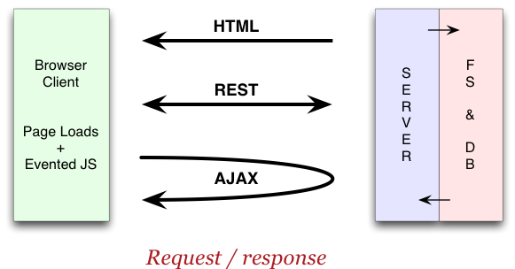
A decade or so ago, this would have been a decent model of how web apps work, I think:

app1

All the pages, styles, images, and some code fetched as HTTP requests, rendered on the server, which sits between the persistent state on the server (files and databases), and the network-facing end.

A RESTful design would then include a clean structure w.r.t how that state on the server is accessed and altered. Then we throw in some behind-the-secnes logic with Ajax to make pages more responsive. This evolved to general-purpose client-side JavaScript libraries like jQuery to get lots of the repetitiveness out of the developer’s workflow. Great stuff.

The assumption here is that servers are big and fast, and that they work reliably, whereas clients vary in capabilities, versions, and performance, and that network connection stability needs to stay out of the “essence” of the application logic.

In a way, it works well. This is the context in which database-backed websites became all the rage: not just a few files and templating to tweak the website, but the essence of the application is stored in a database, with “widgets”, “blocks”, “groups”, and “panes” sewn together by an ever-more elaborate server-side framework – Ruby on Rails, Django, Drupal, etc. WordPress and Redmine too, which I gratefully rely on for the JeeLabs sites.

But there’s something odd going on: a few days ago, the WordPress server VM which runs this daily weblog here at JeeLabs crashed on an out-of-memory error. I used to reserve 512 MB RAM for it, but had scaled it back to 256 MB before the summer break. So 256 MB is not enough apparently, to present a couple of weblog pages and images, and handle some text searches and a simple commenting system.

(We just passed 6000 comments the other day. It’s great to see y’all involved – thanks!)

Ok, so what’s a measly 512 MB, eh?

Well, to me it just doesn’t add up. Ok, so there’s a few hundred MB of images by now. Total. The server is running off an SSD disk, so we should be able to easily serve images with say 25 MB of RAM. But why does WP “need” hundreds of MB’s of RAM to serve a few dozen MB’s of daily weblog posts? Total.

It doesn’t add up. Self-inflicted overhead, for what is 95% a trivial task: serving the same texts and images over and over again to visitors of this website (and automated spiders).

The Redmine project setup is even weirder: currently consuming nearly 700 MB of RAM, yet this ought to be a trivial task, which could probably be served entirely out of say 50 MB of RAM. A tenfold resource consumption difference.

In the context of the home monitoring and automation I’d like to take a bit further, this sort of resource waste is no longer a luxury I can afford, since my aim is to run HouseMon on a very low-end Linux board (because of its low power consumption, and because it really doesn’t do much in terms of computation). Ok, so maybe we need a bit more than 640 KB, but hey… three orders of magnitude?

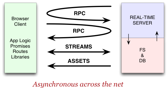
In this context, I think we can do better. Instead of a large server-side byte-shuffling engine, we can now do this – courtesy of modern browsers, Node.js, and AngularJS:

app2

The server side has been reduced to its bare minimum: every “asset” that doesn’t change gets served as is (from files, a database, whatever). This includes HTML, CSS, JavaScript, images, plain text, and any other “document” type blob of information. Nginx is a great example of how a tiny web server based on async I/O and written in C can take care of any load we down-to-earth netizens are likely to encounter.

Let me stress this point: there is no dynamic “templating” or “page generation” on the server side. This takes place in the browser – abstracted away by AngularJS and the DOM.

In parallel, there’s a “Real-Time Server” running, which handles the application logic and everything that needs to be dynamic: configuration! status! measurements! commands! I’m using Node.js, and I’ve started using the fascinating LevelDB database system for all data persistence. The clever bit of LevelDB is that it doesn’t just fetch and store data, it actually lets you keep flows running with changes streamed in and out of it (see the level-livefeed and multilevel projects).

So instead of copying data in and out of a persistent data store, this also becomes a way of staying up to date with all changes on that data. The fusion of a database and pubsub.

On the client side, AngularJS takes care of the bi-directional flow between state (model) and display (view), and Primus acts as generic connection library for getting all this activity across the net – with connection keep-alive and automatic reconnect. Lastly, I’m thinking of incorporating the q-connection library for managing all asynchronicity. It’s fascinating to see network round trip delays being woven into the fabric of an (async / event-driven) JavaScript application. With promises, client/server apps are starting to feel like a single-system application again. It all looks quite, ehm… promising :)

Lots of bits that need to work together. So far, I’m really delighted by the flexibility this offers, and the fact that the server side is getting simpler: just the autonomous data acquisition, a scalable database, a responsive WebSocket server to make the clients (i.e. browsers) come alive, and everything else served as static data. State is confined to the essence of the app. The rest doesn’t change (other than during development of course), needs no big backup solution, and the whole kaboodle should easily fit on a Raspberry Pi – maybe something even leaner than that, one day.

The last instalment tomorrow will be about how HouseMon is structured internally.

PS. I’m not saying this is the only way to go. Just glad to have found a working concoction.

Flow – the developer perspective

In Software on Sep 15, 2013 at 00:01

This is the second of a three-part four-part series on designing big apps (“big” as in not embedded, not necessarily many lines of code – on the contrary, in fact).

Software development is all about “flow”, in two very different ways:

I’ve been looking at lots of options on how to address that first bit, i.e. how to set up an environment which can help me through the edit-run-debug cycle as smoothly and quickly as possible. I didn’t find anything that really fits my needs, so as any good ol’ software developer would do, I scratched this itch recently and ended up creating a new tool.

It’s all about flow. Iterating through the coding process without pushing more buttons or keys than needed. Here’s how it works – there are three kinds of files I need to deal with:

  • HTML – app pages and docs, in the form of Jade and Markdown text files
  • CSS – layout and visual design, in the form of Stylus text files
  • CODE – the logic of it all, host- and client-side, in the form of CoffeeScript text files

Each of these are not the real thing, in the sense that they are all dialects which need to be translated to HTML, CSS, and JavaScript, respectively. But I don’t want a solution which introduces lots of extra steps into that oh-so treasured edit-run-debug cycle of software development. No temporary files, please – let’s generate everything as needed on-the-fly, and let’s set up a single task to take care of it all.

The big issue here is when to do all that pre- (and re-) processing. Again, since staying in the flow is the goal, that really should happen whenever needed and as quickly as possible. The workflow I’ve found to suit me well is as follows:

  • place all the development source files into one nested area (doh!)
  • have the system watch for changes to any files in this area
  • if it’s a HTML file change: reload the browser
  • if it’s a CSS file change: update the browser (no need to reload)
  • if it’s a CODE file change: restart the server and reload the browser

The term for this is “live reload”. It’s been in use for ages by web developers. You save a file, and BAM … the browser updates itself. But that’s only half the story with a client + server setup, as you also may have to restart the server. In the past, I’ve done so using the nodemon utility. It works, but along with other tools too watch for changes and pre-compile to the desired format, it all got a bit clunky.

In the new HouseMon project, it’s all done behind the scenes in a single process. Well, two actually: when in development mode, HouseMon forks itself into a supervisor and a worker child. The supervisor just restarts the worker whenever it exits. And the worker watches for files changes and either reloads or adjusts the browser, or exits. The latter becomes a way for the worker to quickly restart itself from scratch due to a code change.

The result works phenomenally well: I edit in MacVim, multiple files even, and nothing happens. I can bring up the Dash reference guides to look up something. Still nothing happens. But when I switch away from MacVim, it’s set up to save all changes, and everything then kicks in on auto-pilot. Instantly or a few seconds later (depending on the change), the latest changes will be running. The browser may lose a little of its context, but the URL stays the same, so I’m still looking at the same page. The console is open, and I can see what’s going on there. Without ever switching to the browser (ok, I need to switch away from MacVim to something else, but often that will be the command line).

It’s not yet the same as live in-app development (as was possible with Tcl), but it’s getting mighty close, because the app returns to where it was before without pushing any buttons.

There’s one other trick in this setup which is a huge time-saver: whenever the supervisor is launched (“node .“), it scans through all the folders inside the main ./app folder, and collects npm and bower package files as well as Makefile files. All dependencies and requirements are then processed as needed, making the use of 3rd party packages virtually effortless – on the server and in the client. Total automation. Look ma, no hands!

None of this machinery needs to be present in production mode. All this reloading and package dependency handling stuff can then be ignored. Deployment just needs a bunch of static files, served through Node.js, Nginx, Apache, whatever – plus a light-weight Node.js server for the host-side logic, using WebSockets or some fallback mechanism.

As for the big picture on how HouseMon itself is structured… more coming, tomorrow.

Flow – the user perspective

In Software on Sep 14, 2013 at 00:01

This is the first of a three-part four-part series on designing big apps (“big” as in not embedded, not necessarily many lines of code – on the contrary, in fact).

Ok, so maybe what follows is not the user perspective, but my user perspective?

I’m not a fan of pushing clicking buttons. It’s a computer invention, and it sucks.

Interfaces (I’m not keen on the term user interfaces either, but it’s more to the point than just “interfaces”) – anyway, interfaces need interaction to indicate what information you want to see, and to perform a real action, i.e. something that has effect on some permanent state. From setting up preferences or a configuration, to turning on a light.

But apart from that, interaction to fetch or update something is tedious, unwanted, silly, and a waste of time. Pushing a button to see the time is 2,718,281 times more inconvenient than looking at the time. Just like asking for something involves a lot more interaction (and social subtleties) than having the liberty to just do it.

When I look outside the window, I expect to see the actual weather. And when I see information on a screen, I expect it to be up-to-date. I don’t care if the browser does constant refreshes to pull changes from a server or whether it’s set up to respond to push notifications coming in behind the scenes. When I see “22.7°C”, it needs to be a real reading, with a known and acceptable lag and accuracy – unless it’s historical data.

This goes a lot further than numbers and graphs. When I see a button, then to me that is a promise (and invitation) that some action will be taken when I push it. Touch on mobile devices has the advantage here, although clicking via the mouse or typing a power-user keyboard shortcut is often perfectly acceptable – even if slightly more indirect.

What I don’t want is a button which does nothing, or generates an error message. If that button isn’t intended to be used, then it should be disabled or it shouldn’t be there at all:

Screen Shot 2013-09-13 at 11.56.54

Screen Shot 2013-09-13 at 11.57.17

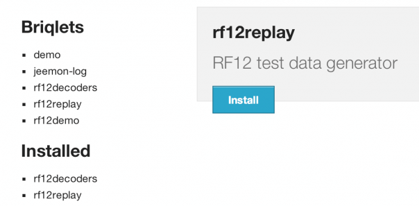
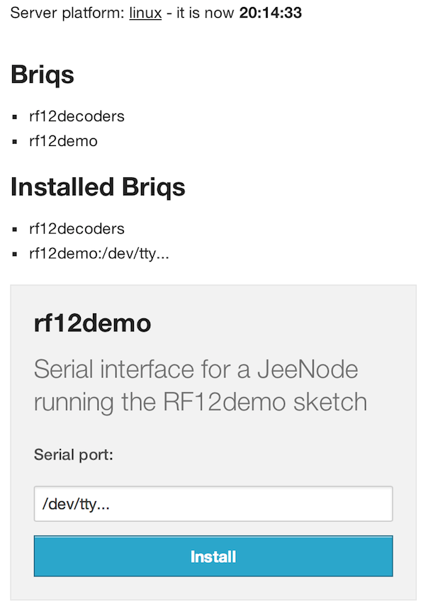
That’s the “Graphs” install page in HouseMon (the wording could have been better).

When a list or graph of readings is shown on-screen, this needs to auto-update in real time. That’s the whole point of HouseMon – access to specific information (that choice is a preference, and will require interaction) to see what’s going on. Now – or within the last few minutes, in the case of sensors which are periodically sending out their readings. A value without an indication of its “up-to-date-ness” is useless. That could be either implicit by displaying it in some special way if the information is stale (slowly turning red?), or explicit, by displaying a time stamp next to it (a bit ugly and tedious).

Would you want it any other way when doing online banking? Would you accept seeing your account balance without guarantee that it is recent?nah, me neither :) – so why do we put up with web pages with copies of some information, at some point in time, getting obsolete the very moment that page is shown?

When “on the web” – as a user – I want to deal with accurate information. When I see something tagged as “updated 2 minutes ago”, then I want to see that “2” change into a “3” within the next minute. See GitHub for an example of this. It works, it makes sense, and it makes the whole technology get out of the way: the web should be an intermediary between some information and me. All the stuff in between is secondary.

Information needs to update – we need to stop copying it into a web page, and send that copy off to the browser. All the lipstick in the world won’t help if what we see is a copy of what we’re looking for. As developers, we need to stop making web sites fancy – we should make them live first and then make them gorgeous. That’s what RIA‘s and SPA‘s are about.

One more thing – not only does information need to flow, these flows should be visualised:

Screen Shot 2013-09-13 at 11.02.15

Such a user interface can be used during development to manage data flows and to design software which ties each result shown on-screen back to its origin. In tomorrow’s apps, every change should propagate – all the way to the pixels shown on-screen by the browser.

Now let’s go back to static web servers to make it happen. Stay tuned…

Gearing up for the new web

In Software on Sep 13, 2013 at 00:01

Well… new for me, anyway. What a fascinating world in motion we live in:

  • first there was the “pre-web”, with email BBS’es and very clunky modem links
  • then came Nestcape Navigator – and the world would never be the same again
  • hey, we can make the results dynamic, let’s generate pages through CGI
  • and not just outgoing, we can have forms and page refreshes to interact!
  • we need lots of ways to generate page variations, let’s add modules to the server
  • nah, we can do better than that: let’s add PHP / Python / Ruby inside the server!
  • and so the first major web explosion of the internet was born…

It took a decade, and another decade to make fast internet access mainstream, which is where we are today. There are lots and lots and LOTS of “web frameworks” in existence now, for any programming language you care about.

The second major wave of evolution came with a whole bunch of new acronyms, such as RIA and SPA. This is very much Google’s turf, and this is the technology which powers Gmail, for example. Rich and responsive interactivity. It’s going everywhere by now.

It was made possible by the super-trio of HTML, CSS, and JS (JavaScript). They’ve all evolved to define the structure, style, and logic of everything you see in the browser.

It’s hard to keep up, but as you know, I’ve picked two very active technologies for doing all my new software development: AngularJS and Node.js. Both by Google, by the way – but also both freely available as wide-open source (here and here). They’ve changed my life :)

It’s been a steep learning curve. I don’t mean just getting something going. I mean getting comfortable with it all. Understanding the idioms and quirks (there always are), and figuring out how to debug stuff (async is nasty, especially when not using promises). Can’t say I’m in the clear yet, but the fog is lifting and the fun level is rising!

I started coding HouseMon many months ago and it’s been running here for a long time now, giving me a chance to let it all sink in. The reality is: I’ve been doing it all wrong.

That’s not necessarily a bad thing, by the way: ya gotta learn stuff by doin’, right?

Ok, so I’ve been using Events as the main decoupling mechanism in HouseMon, i.e. publish and subscribe inside the app. The beauty of this is that it lets you keep the functionality of the application highly modular. Each subsystem subscribes to what it is interested in, and publishes results when they are available. No need to consider who needs this, or even how many subscribers there will be for what gets published.

It sounds great, and in a way it is, but it is a bit like a loose canon: events fire all over the place, with little insight in what is going on and when. For some apps, this is probably great, but with fairly stable continuous processing flows as in a home monitoring setup, it’s more chaotic than need be. It all works fine “in the small”, i.e. when writing little modules (“Briqs” in HouseMon-speak) and adding minor drivers / decoders, but I constantly felt lost with respect to the big picture. And then there’s this nasty back pressure dilemma.

But now the pieces are starting to fall into place. I’ve figured out the “big” structure of the HouseMon application as well as the “little” inner organisation of it all.

It’s all about flow. Three Four stories coming up – stay tuned…

My development setup – utilities

In Software on Sep 12, 2013 at 00:01

As promised, one final post about my development setup – these are all utilities for Mac OSX. There are no doubt a number of equivalents for other platforms. Here’s my top 10:

  • Alfred – Keyboard commands for what normally requires the mouse. I have shortcuts such as cmd-opt-F1 for iTerm, cmd-opt-F2 for MacVim. It launches the app if needed, and then either brings it to the front or hides it. Highly configurable, although I don’t really use that many features – just things like “f blah” to see the list of all folder names matching “blah”. Apart from that, it’s really just an alternative for Spotlight (local disk searches) + Google (or DuckDuckGo) + app launcher. Has earned the #1 keyboard shortcut spot: cmd+space. Top time-saver.

  • HomeBrew – This is the package manager which handles (almost) anything from the Unix world. Installing node.js (w/ npm) is brew install node. Installing MacVim is brew install macvim. Updates too. The big win is that all these installs are compartmentalised, so they can be uninstalled individually as well. Empowering.

  • Dash – Technical reference guides at your fingertips. New guides and updates added a few times a week. Looking for the Date API in JavaScript is a matter of typing cmd-opt-F8 to bring up Dash, and then “js:date”. My developer-pedia.

  • GitHub – Actually, it’s called “GitHub for Mac” – a tool to let you manage all the daily git tasks without ever having to learn the intricacies of git. It handles the 90% most common actions, and it does those well and safely. Push early, push often!

  • SourceTree – Since I’m no git guru, I use SourceTree to help me out with more advanced git actions, with the GUI helping me along and (hopefully) preventing silly mistakes. Every step is trackable, and undoable, but when you don’t know what you’re doing with git, it can become a real mess in the project history. This holds my hand.

  • Dropbox – I’m not into iCloud (too much of a walled garden for me), but for certain things I still need a way to keep things in sync between different machines, and with a few people around the world. Dropbox does that well (though BitTorrent Sync may well replace it one day). Mighty convenient.

  • 1Password – One of the many things that get synced through Dropbox are all my passwords, logins, bank details, and other little secrets. Securely protected by a strong password of course. Main benefit of 1P is that it integrates well with all the browsers, so logging in anywhere, or even coming up with new arbitrary passwords is a piece of cake. Also syncs with mobile. Indispensable.

  • DevonThink – This is my heavyweight external brain. I dump everything in there which needs to be retained. Although plain local search is getting so good and fast that DT is no longer an absolute must, it partitions and organises my files in separate databases (all plain files on disk, so no extra risk of data loss). Intelligent storage.

  • CrashPlan – Nobody should be without (automated, offline) backups. CrashPlan takes care of all the machines around the house. I sleep much better at night because of it. Its only big drawback is that there’s always a 500 MB background process to make this happen (fat Java worker, apparently), and that it burns some serious CPU cycles when checking, or catching up, or cleaning up – whatever. Still, essential.

  • Textual – Yeah, well, ok, this one’s an infrequent member on this list: IRC chat, on the #jeelabs channel for example. Not used much, but when it’s needed, it’s there to get some collaboration done. I’m thinking of hooking this into some sort of personal agents, maybe even have a channel where my house chats about the more public readings coming in. Social, on demand.

The point of all the things I’ve been mentioning in these past few posts, is that it’s all about forming habits, so that a different part of the brain starts doing some of the work for you. There is a perfect French term for getting tools to work for you that way:

  • prolongements du corps (a great example of this is driving a car)

This is my main motivation for adopting touch typing and in particular for using the command-line shell and a keyboard-command based text editor. It (still) doesn’t come easy, but every day I notice some little improvement. As always: Your Mileage May Vary.

Ok, that wraps it up for now. Any other tools you consider really useful? Let me know…

My development setup – software

In Software on Sep 10, 2013 at 00:01

To follow up on yesterday’s post, here are the different software packages in my laptop-based development setup:

  • MacVim is my editor of choice these days. Now that I’ve switched to touch-typing mode, and given that I’ve used vi(m) for as long as I can remember, this is now growing on me every day. It’s all about muscle memory, and off-loading activities to have more spare brain cycles left for the task at hand.

    I chose MacVim over pure vim in the command line for one reason: it can be set to save all files on focus loss, i.e. when switching another app to the foreground. Tried a dark background for a while, but settled on a light one in the end. Dark backgrounds caused trouble with screen reflections when sitting with my back to a window.

  • TextMate is the second editor I use, but exclusively in browse mode. It can be fired up from the command line (e.g. cd housemon && mate .) and makes it very easy to skim and search across large source collections. Having two entirely different contexts means I can keep vim and its history focused on the code I’m actually working on. I only started using this dual-editor approach a few months ago, but by now it’s become a habit to start them both up – on different areas of the screen.

  • Google Chrome is my main development web browser. I settled on it (over Safari) for mostly one reason: it supports having the developer console pane open to the side of the main screen. There are plenty of dev tools included, from browsing the DOM structure to various performance graphs. Using a dedicated browser for development lets me flush the cache and muck with settings without disrupting other web activities.

  • Safari is my secondary browser. This is the one which keeps history, knows how to log into sites, and ends up having lots of tabs and windows open to keep track of all the distractions on the web. Reference docs, searching for information, and all the other time sinks the web has to offer. It drops nicely to the background when I want to get back to the real thing, but it’s there alongside MacVim whenever I need it.

  • iTerm 2 is what I use as command line. The only reason I’m using this instead of the built-in Terminal application, is that it supports split panes (I don’t use screen or tmux much). It’s set up to start up with two windows side-by-side, because tabs are not always convenient: sometimes you really need to see a few things at the same time.

    I do use tabs in all these apps, dragging them around between windows when needed. Sometimes, I’ll open a new iTerm window and make it much larger (all from the keyboard), to see all the output of a ps or grep command, for example.

  • nvAlt is a fork of Notational Velocity – a note-taking app which stores each note as a plain text file. Its main feature is that it starts up and searches everything instantly. Really. In the blink of an eye, I can find all the notes I wrote about anything. I use it for logging how I installed some tricky software and for lots and lots of lists with design ideas. Plain text. Instant. Clickable URLs. Shared through Dropbox. Perfect.

There’s a lot more to it, but these are the six tools I now use day in day out for software development. Even for embedded work, I’ll use the Arduino IDE only as compile + upload step, editing code in MacVim nowadays – because it has so much more functionality.

All of the above are either included in Mac OSX or open source software. I’m inclined to use OSS as a way to keep my learning investments safe. If ever one of these tools ends up going nowhere, or in an unwanted direction, then chances are that some developer(s) will fork the project to keep things on track (as has already happened with TextMate, iTerm, and nvAlt). In the long term, these core tools are simply too important…

My development setup

In Software on Sep 9, 2013 at 00:01

The tools I use for software development have evolved greatly over the years. Some have been replaced, other have simply gotten better, much better, over time. I’d like to describe the setup a bit in the next few posts – and why / how I made those choices. “YMMV”, as they say, but I think it could be of interest to other developers, whether soon-to-be or seasoned-switchers. Context: I develop in (for?) JavaScript (server- and browser-side).

Ok, here goes… the main tools I use are:

  • 2 editors – yes, two…
  • 2 browser – yes, two…
  • 2 command-line windows, yes, two…
  • a note-taking app (sorry, just one :)

Here is a snapshot of all the windows, taken at a fairly arbitrary moment in time:

dev-expose-small

And this is the setup in actual use:

dev-layout-annotated

Tomorrow, I’ll go over the different bits and pieces, and how they work out for me.

My software

In Software on Sep 7, 2013 at 00:01

Most of the software I write, and most of what I’ve written in the past, has gradually been making its way into GitHub. It’s a fantastic free resource for managing code (with no risk of lock-in – ever – since all git history gets copied), and it’s becoming more and more effective at collaboration as well, with a superb issue tracker and excellent searching and statistics facilities. Over the years, each developer home page has evolved into an excellent intro on what he/she has been up to lately:

Screen Shot 2013-09-03 at 14.58.03

As of recently, I’ve turned things up to 11 by giving everyone who submits a pull request full developer access (it’s a manual process, but effortless). As a result, if you submit a pull request, then whenever I merge it into the official repository, I’ll also add you as developer so that you no longer have to fork to get changes in. Just clone the original repo, and push changes back in.

It may sound crazy, but it really isn’t (and it’s not my idea, although I forgot where I first read about it). The point being that contributors are scarce, and good contributors who actually help take a project forward are scarce as gold. Not because there aren’t any, but because few people take the time to actually contribute and participate in a project created by someone else (shame on me for often being like that!). Time is the new scarce resource, so helping others become more productive by not having to go through the pull-request tango to add and tweak stuff really makes sense to me. Let alone giving real credit to people, by not only accepting their gifts but also giving back visibility and responsibility.

I don’t think there is a risk. Every serious developer will check with the team members before committing a contentious or disruptive change, and even then, all it takes is to create a branch and do the work there (while still letting others see what it’s about).

The other change is that I recently discovered the DocumentUp site, which can generate a very nice front page for any project on GitHub, from just its README page – like this one.

This is so convenient that I’ve set up a website with pointers for most of my code:

Screen Shot 2013-09-03 at 13.45.33

There! That URL ought to be fairly easy to remember :)

Another site (service?) which presents (remixes?) GitHub issues in a neat way is waffle.io:

Screen Shot 2013-09-06 at 00.16.16

There’s a lot more going on with GitHub. Did you know that all issue trackers support live chat? Just keep an issue page open, and you’ll see new comments come in – in real time! Perfect for a quick back-and-forth discussion about some intricate problem. Adding images like screen shots is equally easy: just drag and drop the image into the discussion page.

Did you know that each GitHub project can manage releases, either as is or with detailed information per release? Either way, you get a list of versioned ZIP and TAR archives, simply by adding public tags in Git. And even without tagged releases, there’s always a “Download ZIP” link on the right side of each project page, so you don’t even have to install or use git at all to obtain the latest version of that code.

Screen Shot 2013-09-03 at 15.23.37

There are some 4 million public projects on GitHub. Not all exciting, but tons of them are!

Decoding bit fields – part 2

In Software on Sep 6, 2013 at 00:01

To follow up on yesterday’s post, here is some code to extract a bit field. First, a refresher:

bytes5

The field marked in blue is the value we’d like to extract. One way to do this is to “manually” pick each of the pieces and assemble them into the desired form:

bytes4

Here is a little CoffeeScript test version:

buf = new Buffer [23, 125, 22, 2]

for i in [0..3]
  console.log "buf[#{i}] = #{buf[i]} = #{buf[i].toString(2)} b"

x = buf.readUInt32LE 0
console.log "read as 32-bit LE = #{x.toString 2} b"

b1 = buf[1] >> 7
b2 = buf[2]
b3 = buf[3] & 0b111
w = b1 + (b2 << 1) + (b3 << 9)
console.log "extracted from buf: #{w} = #{w.toString 2} b"

v = (x >> 15) & 0b111111111111
console.log "extracted from int: #{v} = #{v.toString 2} b"

Or, if you prefer JavaScript, the same thing:

var buf = new Buffer([23, 125, 22, 2]);

for (var i = 0; i <= 3; ++i) {
  console.log("buf["+i+"] = "+buf[i]+" = "+buf[i].toString(2)+" b");
}

var x = buf.readUInt32LE(0);
console.log("read as 32-bit LE = "+x.toString(2)+" b");

var b1 = buf[1] >> 7;
var b2 = buf[2];
var b3 = buf[3] & 0x7;
var w = b1 + (b2 << 1) + (b3 << 9);
console.log("extracted from buf: "+w+" = "+w.toString(2)+" b");

var v = (x >> 15) & 0xfff;
console.log("extracted from int: "+v+" = "+v.toString(2)+" b");

The output is:

    buf[0] = 23 = 10111 b
    buf[1] = 125 = 1111101 b
    buf[2] = 22 = 10110 b
    buf[3] = 2 = 10 b
    read as 32-bit LE = 10000101100111110100010111 b
    extracted from buf: 1068 = 10000101100 b
    extracted from int: 1068 = 10000101100 b

This illustrates two ways to extract the data: “w” was extracted as described above, but “v” used a trick: first use built-in logic to extract an integer field which is too big (but with all the bits in the right order), then use bit shifting and masking to pull out the required field. The latter is much simpler, more concise, and usually also a little faster.

Here’s an example in Python, illustrating that second approach via “unpack”:

import struct

buf = struct.pack('BBBB', 23, 125, 22, 2)
(x,) = struct.unpack('<l', buf)

v = (x >> 15) & 0xFFF
print(v)

And lastly, the same in Lua, another popular language:

require 'struct'
require 'bit'

buf = struct.pack('BBBB', 23, 125, 22, 2)
x = struct.unpack('<I4', buf)

v = bit.band(bit.rshift(x, 15), 0xFFF)
print(v)

So there you go, lots of ways to extract useful data from the RF12demo sketch output!

Decoding bit fields

In Software on Sep 5, 2013 at 00:01

Prompted by a recent discussion on the forum, and because it’s a recurring theme, I thought I’d go a bit (heh…) into how bit fields work.

One common use-case in Jee-land, is with packets coming in from a roomNode sketch, which are reported by the RF12demo sketch on USB serial as something like:

OK 3 23 125 22 2

The roomNode sketch tightly packs its results into a packet using this C structure:

struct {
    byte light;     // light sensor: 0..255
    byte moved :1;  // motion detector: 0..1
    byte humi  :7;  // humidity: 0..100
    int temp   :10; // temperature: -500..+500 (tenths)
    byte lobat :1;  // supply voltage dropped under 3.1V: 0..1
} payload;

So how do you get the values back out, given just those 4 bytes (plus a header byte)?

To illustrate, I’ll use a slightly more complicated example. But first, some diagrams:

bytes1

bytes2

That’s 4 consecutive bytes in memory, and two ways a 32-bit long int can be mapped to it:

  • little-endian (LE) means that the first byte (at #00) points to the little end of the int
  • big-endian (BE) means that the first byte (at #00) points to the big end of the int

Obvious, right? On x86 machines, and also the ATmega, everything is stored in LE format, so that’s what I’ll focus on from now on (PIC and ARM are also LE, but MIPS is BE).

Let’s use this example, which is a little more interesting (and harder) to figure out:

struct {
    unsigned long before :15;
    unsigned long value :12;  // the value we're interested in
    unsigned long after :3;
} payload;

That’s 30 bits of payload. On an ATmega the compiler will use the layout shown on the left:

bytes3

But here’s where things start getting hairy. If you had used the definition below instead, then you’d have gotten a different packed structure, as shown above on the right:

struct {
    unsigned int before :15;
    unsigned int value :12;  // the value we're interested in
    unsigned int after :3;
} payload;

Subtle difference, eh? The reason for this is that the declared size (long vs int) determines the unit of memory in which the compiler tries to squeeze the bit field. Since an int is 16 bits, and 15 bits were already assigned to the “before” field, the next “value” field won’t fit so the compiler will restart on a fresh byte boundary! IOW, be sure to understand what the compiler does before trying to decode stuff. One way to figure out what’s going on, is to set the values to some distinctive bit patterns and see what comes out as bytes:

payload.before = 0b1;  // bit 0 set
payload.value = 0b11;  // bits 0 and 1 set
payload.after = 0b111; // bits 0, 1, and 2 set

Tomorrow, I’ll show a couple of ways to extract this bit field.

Back pressure

In Software on Sep 4, 2013 at 00:01

No, not the medical term, and not this carambolage either (though it’s related):

52-car-pile-up

What I’m talking about is the software kind: back pressure is what you need in some cases to avoid running into resource limits. There are many scenario’s where this can be an issue:

  • In the case of highway pile-ups, the solution is to add road signalling, so drivers can be warned to slow down ahead of time – before that decision is taken from them…
  • Sending out more data than a receiver can handle – this is why traditional serial links had “handshake” mechanisms, either software (XON/XOFF) or hardware (CTS/RTS).
  • On the I2C bus, hardware-based clock stretching is often supported as mechanism for a slave to slow down the master, i.e. an explicit form of back pressure.
  • Sending out more packets than (some node in) a network can handle – which is why backpressure routing was invented.
  • Writing out more data to the disk than the driver/controller can handle – in this case, the OS kernel will step in and suspend your process until things calm down again.
  • Bringing a web server to its knees when it gets more requests than it can handle – crummy sites often suffer from this, unless the front end is clever enough to reject requests at some point, instead of trying to queue more and more work which it can’t possibly ever deal with.
  • Filling up memory in some dynamic programming languages, where the garbage collector can’t keep up and fails to release unused memory fast enough (assuming there is any memory to release, that is).

That last one is the one that bit me recently, as I was trying to reprocess my 5 years of data from JeeMon and HouseMon, to feed it into the new LevelDB storage system. The problem arises, because so much in Node.js is asynchronous, i.e. you can send off a value to another part of the app, and the call will return immediately. In a heavy loop, it’s easy to send off so much data that the callee never gets a chance to process it all.

I knew that this sort of processing would be hard in HouseMon, even for a modern laptop with oodles of CPU power and gigabytes of RAM. And even though it should all run on a Raspberry Pi eventually, I didn’t mind if reprocessing one year of log files would take, say, an entire day. The idea being that you only need to do this once, and perhaps repeat it when there is a major change in the main code.

But it went much worse than I expected: after force-feeding about 4 months of logs (a few hundred thousand converted data readings), the Node.js process RAM consumption was about 1.5 GB, and Node.js was frantically running its garbage collector to try and deal with the situation. At that point, all processing stopped with a single CPU thread stuck at 100%, and things locked up so hard that Node.js didn’t even respond to a CTRL-C interrupt.

Now 1.5 GB is a known limit in the V8 engine used in Node.js, and to be honest it really is more than enough for the purposes and contexts for which I’m using it in HouseMon. The problem is not more memory, the problem is that it’s filling up. I haven’t solved this problem yet, but it’s clear that some sort of back pressure mechanism is needed here – well… either that, or there’s some nasty memory leak in my code (not unlikely, actually).

Note that there are elegant solutions to this problem. One of them is to stop having a producer push data and calls down a processing pipeline, and switch to a design where the consumer pulls data when it is ready for it. This was in fact one of the recent big changes in Node.js 0.10, with its streams2 redesign.

Even on an embedded system, back pressure may cause trouble in software. This is why there is an rf12_canSend() call in the RF12 driver: because of that, you cannot ever feed it more packets than the (relatively slow) wireless RFM12B module can handle.

Soooo… in theory, back pressure is always needed when you have some constraint further down the processing pipeline. In practice, this issue can be ignored most of the time due to the slack present in most systems: if we send out at most a few messages per minute, as is common with home monitoring and automation, then it is extremely unlikely that any part of the system will ever get into any sort of overload. Here, back pressure can be ignored.

Electricity usage patterns

In Hardware, Software on Sep 3, 2013 at 00:01

Given that electricity usage here is monitored with a smart meter which periodically phones home to the electricity company over GPRS, this is the sort of information they get to see:

Screen Shot 2013-09-02 at 11.20.38

Consumption in blue, production in green. Since these are the final meter readings, those two data series will never overlap – ya can’t consume and produce at the same time!

I’m reading out the P1 data and transmitting it wirelessly to my HouseMon monitoring setup (be sure to check the develop branch, which is where all new code is getting added).

There’s a lot of information to be gleaned from that. The recurring 2000+ W peaks are from a 7-liter kitchen boiler (3 min every 2..3 hours). Went out for dinner on Aug 31st, so no (inductive) home cooking, and yours truly burning lots of midnight oil into Sep 1st. Also, some heavy-duty cooking on the evening of the 1st (oven dish + stove).

During the day, it’s hard to tell if anyone is at home, but evenings and nights are fairly obvious (if only by looking at the lights lit in the house!). Here’s Sep 2nd in more detail:

Screen Shot 2013-09-02 at 11.23.50

This one may look a bit odd, but that double high-power blip is the dish washer with its characteristic two heating cycles (whoops, colours reversed: consumption is green now).

Note that whenever there is more sun, there would be fewer consumption cycles, and hence less information to glean from this single graph. But by matching this up with other households nearby, you’d still get the same sort of information out, i.e. from known solar power vs. returned power from this household. Cloudy patterns will still match up across a small area (you can even determine the direction of the clouds!).

I don’t think there’s a concern for (what little) privacy (we have left), but it’s quite intriguing how much can be deduced from this.

Here’s yet more detail, now including the true house usage and solar production values, as obtained from some pulse counters, this hardware and the homePower driver:

Screen Shot 2013-09-02 at 11.52.21

There is a slight lag in smart meter reporting (a value on the P1 port every 10s). This is not an issue of the smart meter though: the DyGraphs package is only able to plot step lines with values at the start of the step, even though these values pertain to the past 10 seconds.

Speaking of which – there was a problem with the way data got stored in Redis. This is no longer an issue in this latest version of HouseMon, because I’m switching over to LevelDB, a fascinating time- and space-efficient database engine.

FanBot Registration System

In Software, Linux on Jun 29, 2013 at 00:01

Nearly 400 FanBots have already been built – see this page and the KekBot weblog.

To finish this little series, I wanted to describe the little setup I built and how it was done. Nothing spectacular, more an example of how you can create a software cocktail / mashup to get a one-off short-lived project like this going fast.

First the basic task at hand: allow kids to register their FanBot and print out a “passport” with a picture of their creation and some information about when and how to get their FanBot back after the RoboCup 2013 event. At the same time, it would be nice to have a monitor display the current count and show images of the last few FanBot pictures taken.

passport

I decided to use 3 Raspberry Pi’s as “slave”, each with a webcam, an LCD screen (thanks David, for the laser-cut frame!), and Ethernet + power. The code running on them is on github. It would be nice if each slave could continue to accept registrations even with the network connection temporarily down, so I went for the following approach:

  • collect registrations locally, using rsync to push new ones to the master
  • everything is based on a few simple shell scripts for quick adjustment
  • two C/C++ programs were needed: to read the FanBot data and to drive the LCD
  • do a git pull on power-up and re-compile as needed before starting operation
  • periodic webcam readout and periodic rsync, using loops and sleep calls

For the master, I thought about using the Odroid/U2, but decided against it as there would be too much setup involved in the last minute. Next idea was to use an Acer Inspire One Linux netbook, but it turned out to be way too slow. For some reason, Node.js was consuming 100% CPU (I suspect a bad nodemon disk change polling error on the slow SSD). No time to figure that out, so I ended up using my second Mac laptop instead.

The master logic started out as follows:

  • an rsync server was set up to collect files from all the slaves in one spot
  • the display is presented via a browser in full-screen mode and Node.js
  • the original plan was to also allow outside access, but we never got to that
  • for live updating, I decided to use SocketStream (same as in HouseMon)
  • a PDF was generated for each image by convert, which is part of ImageMagick
  • an AppleScript then prints each PDF to the USB-attached laser-printer

These choices turned out to be very convenient: by having the rsync folder inside the Node.js application area, and using nodemon, refresh became automatic (nodemon + socketstream will force a refresh on each client whenever a file system change is detected). So all I had to do was write a static Node.js app to display the count and the latest images.

So far so good. A couple of glitches, such as an erratic printer (new firmware fixed it), an overheating RPi (fixed by clocking at 700 MHz again), and all the slave rsyncs fighting when the same registration was present on more than one (fixed by adding the “-u” flag).

During installation, we found out that there was no wired ethernet w/ DHCP, as I had assumed. Oops. So the Mac laptop was turned into a WiFi -> wired bridge, since WiFi was available most of the time. Whoops: “most” is not good enough, the RPi’s have no clock, they really need an NTP server – especially since the whole system was based on rsync and file modification times! We hacked a fixed DNS – but internet still has to be there.

And then the fun started – various little wishes came up after the fact:

  • can we get images + passports off-site during the event? sure: rsync them to Dropbox
  • could we have a page with all images? sure: on my server at JeeLabs, I made an rsync loop from one Dropbox area to another, and made a little photo-album using Dropbox
  • could we show a live count, even though the monitor website was not accessible? sure: I simply added another shell loop on my server again, to generate an image with the count in it, and made it show up as first one in the photo album.

Here is the shell script for that last feature:

cd ~/Dropbox/FanBots
while :
do
  N=$(echo `ls *.jpg | wc -l`)
  if [ "$N" != "$P" ]
  then
    echo $N - `date`
    convert -background black -fill red -size 480x640 \
      -gravity center "label:$N\n\nFanBots" 0-teller.png
    P=$N
  fi
  sleep 10
done

This can run anywhere, since Dropbox is taking care of all updates in both directions!

The point of all this is not which languages I used (your choice will definitely be superior), nor what hardware was selected for this (it changed several times). The point is that:

  1. it all got done in a very limited amount of time
  2. the basic rsync approach made things resilient and self-recovering
  3. github pulls made it possible to apply last-minute tweaks
  4. some nice changes were possible very late in the game
  5. dropbox integration made it possible to add features remotely

Happy ending: all the kids are having a good time … including me :)

PS. Tomorrow (Sunday) is the RoboCup 2013 finals. See you there?

Packaged but not virtualised

In Hardware, Software, Linux on Jun 26, 2013 at 00:01

Since VMware started virtualising x86 hardware many years ago, many uses have been found for this approach of creating fully self-contained software environments. I’ve used VMware many years, and was pleased when Apple switched the Macs to “Intel inside”.

Nowadays, I can run numerous variants of Windows as well as Linux on a single laptop. I switched to Parallels as VM core, but the principle remains the same: a large file is used as virtual hard disk, with an operating system installed, and from then on the whole environment simply “runs” inside the Mac host (in my case).

Nowadays, we all take this for granted, and use virtual environments as ultra-low cost web servers without even giving it any thought. I have a number of virtual machines running on a Mac Mini for all the JeeLabs sites in fact (and some more). One piece of hardware, able to suspend and resume N completely independent systems at the click of a mouse.

But there’s a drawback: you end up duplicating a lot of the operating system and main services in each VM, and as a result this stuff not only consumes disk space but also leads to a lot of redundant backup data. I keep the VM’s very lean and mean here, but they still all eat up between 3 and 10 gigbytes of disk space. Doesn’t sound like much, but I’m pretty sure my own data uses less than 10% of that space…

Both Parallels and VMware (and probably also VirtualBox) support snapshotting, which means that in principle you could set up a full Linux environment with a LAMP stack, and then use snapshots to only store what’s different for each VM. But that’s not useful in the long run, because as soon as you get system updates, they’ll end up being duplicated again.

It’s a bit like git “forks”: set up a state, create a fork to create a variant, and then someone decides to add some features (or fix some bugs) to the original which you’d also like to adopt. For git, the solution is to merge the original changes into your fork, and use “fast-forwarding” (if I understand it correctly – it’s all still pretty confusing stuff).

So all in all, I think VM’s are really brilliant… but not always convenient. Before you know it, you end up maintaining and upgrading N virtual machines every once in a while.

I’ve been using TurnkeyLinux as basis of all my VM’s because they not only maintain a terrific set of ready-to-run VM images, but because they also make them self-updating out of the box, and because they’ve added a very convenient incremental daily backup mechanism which supports restarting from the back-up. You can even restart in the cloud, using Amazon’s EC2 VM “instances”.

And then someone recently told me about Docker – “The Linux container engine”.

This is a very interesting new development. Instead of full virtualisation, it uses “chroot” and overlay file systems to completely isolate code from the rest of the 64-bit Linux O/S it is running on. This lets you create a “box” which keeps every change inside.

My view on this, from what I understand so far, is that Docker lets you play git at the operating system level: you take a system state, make changes to it, and then commit those changes. Not once, but repeatedly, and nested to any degree.

The key is the “making changes” bit: you could take a standard Linux setup as starting point (Docker provides several base boxes), install the LAMP stack (if someone hasn’t done this already), commit it, and then launch that “box” as web server. Whereby launching could include copying some custom settings in, running a few commands, and then starting all the services.

The way to talk to these Docker boxes is via TCP/IP connections. There’s also a mechanism to hook into stdin/stdout, so that you can see logs and such, or talk to an interactive shell inside the box, for example.

The difference with a VM, is that these boxes are very lightweight. You can start and stop them as quickly as any other process. Lots of ’em could be running at the same time, all within a single Linux O/S environment (which may well be a VM, by the way…).

Another example would be to set up a cross compiler for AVR’s/Arduino’s (or ARMs) as a box in Docker. Then a compile would be: start the box, feed it the source files, get the results out, and then throw the box away. Sounds a bit drastic, but it’s really the same as quitting an application – which throws all the state in RAM away. The point is that now you’re also throwing away all the uninteresting side-effects accumulated inside the box!

I haven’t tried out much so far. Docker is very new, and I need to wrap my mind around it to really understand the implications, but my hunch is that it’s going to be a game changer. With the same impact on computation and deployment as VMware had at the time.

As with VM’s, Docker boxes can be saved, shared, moved around, and launched on different machines and even different environments.

For more info, see this page which draws an analogy with freight containers, and how one standard container design has revolutionised the world of shipping and freight / cargo handling. I have this feeling that the analogy is a good one… a fascinating concept!

Update – Here’s a nice example of running a Node.js app in Docker.

FanBots at RoboCup 2013

In Hardware, Software, Linux, ARM on Jun 25, 2013 at 00:01

There’s an event coming up in a few days in Eindhoven, called the RoboCup 2013:

teun

This is the world championship of robotic football. For all ages, and with various levels of sophistication. Some robots are tiny cars, trying to work together to play a match, some robots are little human-like machines consisting of lots of servos to make them walk on two feet, and some robots are very sophisticated little “towers” on three wheels, zipping along at impressive speeds and able to catch, hold, and kick a standard-size football.

I’m not directly involved in this, but I saw some of the preparations and it really promises to be a fantastic event. Lots of geeks with laptops, soldering irons, and mechanical stuff. The kick-off is next Wednesday and the event lasts for five days, with the finals on Sunday.

On the side, there is a gorgeous (not-so) little project going on, whereby kids of ages 8 to 12 can visit a workshop to build their own FanBot (for free). The FanBot can blink its eyes and mouth, and wave its arms – part of the exercise is to create a little “program” of things it does at the press of a button, so this will also be a first encounter with programming!

There’s a Dutch page about the project and a general page in English mentioning FanBots.

But the really exciting goal will be to create a huge stand for all the FanBots and make them cheer the football-playing robots in the main event hall. The aim is to get up to 1000 of them, all blinking and waving – and all orchestrated and controlled from a central system. It’s all being designed and built by Peter Brier and by Marieke Peelen of KekkeTek.

One task in the project is to register all the FanBots and print out a little “passport” as last step – which the kids can then use to pick up their own FanBot once the RoboCup 2013 event is over. This is the part I volunteered to help with.

I’ll describe the setup in more detail soon, but that’s where the Raspberry Pi’s w/ LCD screen and webcams will be used. It’ll be fun to see whether we can get 1000 kids to build and sign up their little robots during three days – there’s quite a bit of logistics involved!

Admission is free, so if you’re in the neighbourhood: don’t miss it – it’s going to be fun!

Fast I/O on a Raspberry Pi

In Hardware, Software, Linux on Jun 15, 2013 at 00:01

To follow up on yesterday’s post about WiringPi and how it was used to display an image on a colour LCD screen attached to the RPi via its GPIO pins.

A quick calculation indicated that the WiringPi library is able to toggle the GPIO pins millions of times per second. Now this might not seem so special if you are used to an ATmega328 on a JeeNode or other Arduino-like board, but actually it is

Keep in mind that the RPi code is running under Linux, a multi-tasking 32-bit operating system which not only does all sorts of things at (nearly) the same time, but which also has very solid memory and application protection mechanisms in place:

  • each application runs in its own address space
  • the time each application runs is controlled by Linux, not the app itself
  • applications can crash, but they cannot cause the entire system to crash
  • dozens, hundreds, even thousands of applications can run next to each other
  • when memory is low, Linux can swap some parts to disk (not recommended with SD’s)

So while the LCD code works well, and much faster than one might expect for all the GPIO toggling it’s doing, this isn’t such a trivial outcome. The simplest way to deal with the RPi’s GPIO pins, is to manipulate the files and directories under the /sys/class/gpio/ “device tree”. This is incredibly useful because you can even manipulate it via plain shell script, using nothing but the “echo”, “cat”, and “ls” commands. Part of the convenience is the fact that these manipulations can take place entirely in ASCII, e.g. writing the string “1” or “0” to set/reset GPIO pins.

But the convenience of the /sys/class/gpio/ virtual file system access comes at a price: it’s not very fast. There is too much involved to deal with individual GPIO pins as files!

WiringPi uses a different approach, called “memory mapped files”.

Is it fast? You bet. I timed the processing time of this snippet of C code:

int i;
for (i = 0; i < 100000000; ++i) {
  digitalWrite(1, 1);
  digitalWrite(1, 0);
}
return 0;

Here’s the result:

    real    0m19.592s
    user    0m19.490s
    sys     0m0.030s

That’s over 5 million pulses (two toggles) per second.

This magic is possible because the I/O address space (which is normally completely inaccessible to user programs) has been mapped into a section of the user program address space. This means that there is no operating system call overhead involved in toggling I/O bits. The mapping is probably virtualised, i.e. the kernel will kick in on each access, but this is an interrupt straight into protected kernel code, so overhead is minimal.

How minimal? Well, it takes less than 90 ns per call to digitalWrite(), so even when running at the RPi’s maximum 1 GHz rate, that’s less than 90 machine cycles.

Note how the RPi can almost toggle an I/O pin as fast as an ATmega running at 16 MHz. But the devil is in the details: “can” is the keyword here. Being a multi-tasking operating system, there is no guarantee whatsoever that the GPIO pin will always toggle at this rate. You may see occasional hick-ups in the order of milliseconds, in fact.

Is the RPi fast? Definitely! Is it guaranteed to be fast at all times? Nope!

What it took to generate that LCD image

In Hardware, Software, Linux on Jun 14, 2013 at 00:01

As shown yesterday, it’s relatively easy to get a bitmap onto an LCD screen connected to a few I/O pins of the Raspberry Pi.

But there were some gotcha’s:

  • the image I wanted to use was 640×480, but the LCD is only 320×240 pixels
  • the WiringPi library has code to put a bitmap on the screen, but not JPEGs
  • this is easy to fix using the ImageMagick “convert” command
  • but the result has 24-bit colour depth, whereas the LCD wants 16-bit (5-6-5)

The “convert” command makes things very easy, but first I had to install ImageMagick:

    sudo apt-get install ImageMagick

Then we can run “convert” from the command-line (long live the Unix toolkit approach!):

    convert snap.jpg -geometry 320x240 -normalize snap.rgb

This handles both the rescaling and the transformation to a file with (R,G,B) types, each colour is one byte. As expected, the resulting image file is 320 x 240 x 3 = 230,400 bytes.

I didn’t see a quick way to convert the format to the desired 5-6-5-bit coding needed for the LCD, and since the code to write to the LCD is written in C anyway (to link to WiringPi), I ended up doing it all in a straightforward loop:

#define PIXELS (320*240)
uint8_t rgbIn24 [PIXELS][3];
unsigned rgbOut15 [PIXELS];

[...]

for (x = 0; x < PIXELS; ++x) {
  uint8_t r = rgbIn24[x][0] >> 3;
  uint8_t g = rgbIn24[x][1] >> 2;
  uint8_t b = rgbIn24[x][2] >> 3;
  rgbOut15[x] = (r << 11) | (g << 5) | b;
}

Note that this is a C program compiled and running under Linux on the RPi, and that it can therefore easily allocate some huge arrays. This isn’t some tiny embedded 8-bit µC with a few kilobytes – it’s a full-blown O/S running on a 32-bit CPU with virtual memory!

The other gotcha was that the bitmap to be supplied to the LCD library on top of WiringPi was expected to store each pixel in a 32-bit int. Total waste of space, and probably the result of a rushed port from the UTFT code (written to assume 16-bit ints) to the RPi. Which is why rgbOut15 is declared as “unsigned” (int, i.e. uint32_t) array, although the image really only needs an uint16_t. Oh well, what’s an extra 150 kB, eh?

Anyway, it works. Perfection can wait.

Note that this sends out all the data pixel by pixel to the display, and that each pixel takes the bit-banging of 2 bytes (the interface to the LCD is 8-bit wide), so each pixel takes at least 20 calls to digitalWrite(): 8 to set the data bits, and 2 two to toggle a clock pin – times two for the 2 bytes per pixel. That’s at least 4.6 million GPIO pin settings in half a second!

Tomorrow, I’ll show how WiringPi can make GPIO pins change in under 100 nanoseconds.

Idling in low-power mode

In AVR, Software on May 28, 2013 at 00:01

With a real-time operating system, going into low-power mode is easy. Continuing the recent ChibiOS example, here is a powerUse.ino sketch which illustrates the mechanism:

#include <ChibiOS_AVR.h>
#include <JeeLib.h>

const bool LOWPOWER = true; // set to true to enable low-power sleeping

// must be defined in case we're using the watchdog for low-power waiting
ISR(WDT_vect) { Sleepy::watchdogEvent(); }

static WORKING_AREA(waThread1, 50);

void Thread1 () {
  while (true)
    chThdSleepMilliseconds(1000);
}

void setup () {
  rf12_initialize(1, RF12_868MHZ);
  rf12_sleep(RF12_SLEEP);

  chBegin(mainThread);
}

void mainThread () {
  chThdCreateStatic(waThread1, sizeof (waThread1),
                    NORMALPRIO + 2, (tfunc_t) Thread1, 0);

  while (true)
    loop();
}

void loop () {
  if (LOWPOWER)
    Sleepy::loseSomeTime(16); // minimum watchdog granularity is 16 ms
  else
    delay(16);
}

There’s a separate thread which runs at slightly higher priority than the main thread (NORMALPRIO + 2), but is idle most of the time, and there’s the main thread, which in this case takes the role of the idling thread.

When LOWPOWER is set to false, this sketch runs at full power all the time, drawing about 9 mA. With LOWPOWER set to true, the power consumption drops dramatically, with just an occasional short blip – as seen in this current-consumption scope capture:

SCR35

Once every 16..17 ms, the watchdog wakes the ATmega out of its power-down mode, and a brief amount of activity takes place. As you can see, most of these “blips” take just 18 µs, with a few excursions to 24 and 30 µs. I’ve left the setup running for over 15 minutes with the scope background persistence turned on, and there are no other glitches – ever. Those 6 µs extensions are probably the milliseconds clock timer.

For real-world uses, the idea is that you put all your own code in threads, such as Thread1() above, and call chThdSleepMilliseconds() to wait and re-schedule as needed. There can be a number of these threads, each with their own timing. The lowest-priority thread (the main thread in the example above) then goes into a low-power sleep mode – briefly and repeatedly, thus “soaking” up all unused µC processor cycles in the most energy-efficient manner, yet able to re-activate pending threads quickly.

What I don’t quite understand yet in the above scope capture is the repetition frequency of these pulses. Many pulses are 17 µs apart, i.e. the time Sleepy::loseSomeTime() goes to sleep, but there are also more frequent pulses, spread only 4..9 ms apart at times. I can only guess that this has something to do with the ChibiOS scheduler. That’s the thing with an RTOS: reasoning about the repetitive behavior of such code becomes a lot trickier.

Still… not bad: just a little code on idle and we get low-power behaviour almost for free!

ChibiOS for the Arduino IDE

In AVR, Software on May 25, 2013 at 00:01

A real-time operating system is a fairly tricky piece of software, even with a small RTOS – because of the way it messes with several low-level details of the running code, such as stacks and interrupts. It’s therefore no small feat when everything can be done as a standard add-on library for the Arduino IDE.

But that’s exactly what has been done by Bill Greiman with ChibiOS, in the form of a library called “ChibiOS_AVR” (there’s also an ARM version for the Due & Teensy).

So let’s continue where I left off yesterday and install this thing for use with JeeNodes, eh?

  • download a copy of ChibiOS20130208.zip from this page on Google Code
  • unpack it and inside you’ll find a folder called ChibiOS_AVR
  • move it inside the libraries folder in your IDE sketches folder (next to JeeLib, etc)
  • you might also want to move ChibiOS_ARM and SdFat next to it, for use later
  • other things in that ZIP file are a README file and the HTML documentation
  • that’s it, now re-launch the Arduino IDE to make it recognise the new libraries

That’s really all there is to it. The ChibiOS_AVR folder also contains a dozen examples, each of which is worth looking into and trying out. Keep in mind that there is no LED on a standard JeeNode, and that the blue LED on the JeeNode SMD and JeeNode USB is on pin 9 and has a reverse polarity (“0” will turn it on, “1” will turn it off).

Note: I’m using this with Arduino IDE 1.5.2, but it should also work with IDE 1.0.x

Simple things are still relatively simple with a RTOS, but be prepared to face a whole slew of new concepts and techniques when you really start to dive in. Lots of ways to make tasks and interrupts work together – mutexes, semaphores, events, queues, mailboxes…

Luckily, ChibiOS comes with a lot of documentation, including some general guides and how-to’s. The AVR-specific documentation can be found here (as well as in that ZIP file you just downloaded).

Not sure this is the best place for it, but I’ve put yesterday’s example in JeeLib for now.

I’d like to go into RTOS’s and ChibiOS some more in the weeks ahead, if only to see how wireless communication and low-power sleep modes can be fitted in there.

Just one statistic for now: the context switch latency of ChibiOS on an ATmega328 @ 16 MHz appears to be around 15 µs. Or to put it differently: you can switch between multiple tasks over sixty thousand times a second. Gulp.

Blinking in real-time

In AVR, Software on May 24, 2013 at 00:01

As promised yesterday, here’s an example sketch which uses the ChibiOS RTOS to create a separate task for keeping an LED blinking at 2 Hz, no matter what else the code is doing:

#include <ChibiOS_AVR.h>

static WORKING_AREA(waThread1, 50);

void Thread1 () {
  const uint8_t LED_PIN = 9;
  pinMode(LED_PIN, OUTPUT);
  
  while (1) {
    digitalWrite(LED_PIN, LOW);
    chThdSleepMilliseconds(100);
    digitalWrite(LED_PIN, HIGH);
    chThdSleepMilliseconds(400);
  }
}

void setup () {
  chBegin(mainThread);
}

void mainThread () {
  chThdCreateStatic(waThread1, sizeof (waThread1),
                    NORMALPRIO + 2, (tfunc_t) Thread1, 0);
  while (true)
    loop();
}

void loop () {
  delay(1000);
}

There are several things to note about this approach:

  • there’s now a “Thread1” task, which does all the LED blinking, even the LED pin setup
  • each task needs a working area for its stack, this will consume a bit of memory
  • calls to delay() are forbidden inside threads, they need to play nice and go to sleep
  • only a few changes are needed, compared to the original setup() and loop() code
  • chBegin() is what starts the RTOS going, and mainThread() takes over control
  • to keep things similar to what Arduino does, I decided to call loop() when idling

Note that inside loop() there is a call to delay(), but that’s ok: at some point, the RTOS runs out of other things to do, so we might as well make the main thread similar to what the Arduino does. There is also an idle task – it runs (but does nothing) whenever no other tasks are asking for processor time.

Note that despite the delay call, the LED still blinks in the proper rate. You’re looking at a real multitasking “kernel” running inside the ATmega328 here, and it’s preemptive, which simply means that the RTOS can (and will) decide to break off any current activity, if there is something more important that needs to be done first. This includes suddenly disrupting that delay() call, and letting Thread1 run to keep the LEDs blinking.

In case you’re wondering: this compiles to 3,120 bytes of code – ChibiOS is really tiny.

Stay tuned for details on how to get this working in your projects… it’s very easy!

It’s time for real-time

In Software on May 23, 2013 at 00:01

For some time, I’ve been doodling around with various open-source Real-time operating system (RTOS) options out there. There are quite a few out there to get lost in…

But first, what is an RTOS, and why would you want one?

The RTOS is code which can manage multiple tasks in a computer. You can see what it does by considering what sort of code you’d write if you wanted to periodically read out some sensors, not necessarily all at the same time or equally often. Then, perhaps you want to respond to external events such as a button press of a PIR sensor firing, and let’s also try and report this on the serial port and throw in a command-line configuration interface on that same serial port…

Oh, and in between, let’s go into a low-power mode to save energy.

Such code can be written without RTOS, in fact that’s what I did with a (simpler) example for the roomNode sketch. But it gets tricky, and everything can become a huge tangle of variables, loops, conditions, and before you know it … you end up with spaghetti!

In short, the problem is blocking code – when you write something like this, for example:


void setup () {}

void loop () {
  digitalWrite(LED, HIGH);
  delay(100);
  digitalWrite(LED, LOW);
  delay(400);
}

The delay() calls will put the processor into a busy loop for as long as needed to make the requested number of milliseconds pass. And while this is the case, nothing else can be done by the processor, other than handling hardware interrupts (such as timer ticks).

What if you wanted to respond to button presses? Or make a second LED blink at a different rate at the same time? Or respond to commands on the serial port?

This is why I added a MilliTimer class to JeeLib early on. Let’s rewrite the code:


MilliTimer ledTimer;
bool ledOn;;

void setup () {
  ledTimer.set(1); // start the timer
}

void loop () {
  if (ledTimer.poll()) {
    if (ledOn) {
      digitalWrite(LED, LOW);
      ledTimer.set(400);
    } else {
      digitalWrite(LED, HIGH);
      ledTimer.set(100);
    }
    ledOn = ! ledOn;
  }
  // anything ...
}

It’s a bit more code, but the point is that this implementation is no longer blocking: instead of stopping on a delay() call, we now track the progress of time through the MilliTimer, we keep track of the LED state, and we adjust the time to wait for the next change.

As a result, the comment line at the end gets “executed” all the time, and this is where we can now perform other tasks while the LED is blinking in the background, so to speak.

You can get a lot done this way, but things do tend to become more complicated. The simple flow of each separate activity starts to become a mix of convoluted flows.

With a RTOS, you can create several tasks which appear to all run in parallel. You don’t call delay(), but you tell the RTOS to suspend your task for a certain amount of time (or until a certain event happens, which is the real magic sauce of RTOS’es, actually).

So in pseudo code, we can now write our app as:

  TASK 1:
    turn LED on
    wait 100 ms
    turn LED off
    wait 400 ms
    repeat

  MAIN:
    start task 1
    do other stuff (including starting more tasks)

All the logic related to making the LED blink has been moved “out of the way”.

Tomorrow I’ll expand on this, using an RTOS which works fine in the Arduino IDE.

Tricky graphs – part 2

In Software on May 20, 2013 at 00:01

As noted in a recent post, graphs can be very tricky – “intuitive” plots are a funny thing!

Screen Shot 2013-05-14 at 10.35.43

I’ve started implementing the display of multiple series in one graph (which is surprisingly complex with Dygraphs, because of the way it wants the data points to be organised). And as you can see, it works – here with solar power generation measured two different ways:

  • using the pulse counter downstairs, reported up to every 3 seconds (green)
  • using the values read out from the SB5000TL inverter via Bluetooth (blue)

In principle, these represent the same information, and they do match more-or-less, but the problem mentioned before makes the rectangles show up after each point in time:

Screen Shot 2013-05-14 at 10.40.11

Using a tip from a recent comment, I hacked in a way to shift each rectangle to the left:

Screen Shot 2013-05-14 at 10.40.34

Now the intuition should be that the area in the coarser green rectangles should be the same as the blue area they overlap. But as you can see, that’s not the case. Note that the latter is the proper way to represent what was measured: a measurement corresponds to the area preceding it, i.e. that hack is an improvement.

So what’s going on, eh?

Nice puzzle. The explanation is that the second set of readings is incomplete: the smaRelay sketch only obtains a reading from the inverter ever 5 minutes or so, but that’s merely an instantaneous power estimate, not an averaged reading since the previous readout!

So there’s not really enough data in the second series to produce an estimate over each 5-minute period. All we have is a sample of the power generation, taken once every so often.

Conclusion: there’s no way to draw the green rectangles to match our intuition – not with the data as it is being collected right now anyway. In fact, it’ probably more appropriate to draw an interpolated line graph for that second series, or better still: dots

Update – Oops, the graphs are coloured differently, my apologies for the extra confusion.

Measurement intervals and graphs

In Software on May 13, 2013 at 00:01

One more post about graphs in this little mini-series … have a look at this example:

Screen Shot 2013-05-10 at 19.33.51

Apart from some minor glitches, it’s in fact an accurate representation of the measurement data. Yet there’s something odd: some parts of the graph are more granular than others!

The reason for this is actually completely unrelated to the issues described yesterday.

What is happening is that the measurement is based on measuring the time between pulses in my pulse counters, which generate 2000 pulses per kWh. A single pulse represents 0.5 Wh of energy. So if we get one pulse per hour, then we know that the average consumption during that period was 0.5 W. And when we get one pulse per second, then the average (but near-instantaneous) power consumption over that second must have been 1800 W.

So the proper way to calculate the actual power consumption, is to use this formula:

    power = 1,800,000 / time-since-last-pulse-in-milliseconds

Which is exactly how I’ve been measuring power for the past few years here at JeeLabs. The pulses represent energy consumption (i.e. kWh), whereas the time between pulses represents estimated actual power use (i.e. W).

This type of measurement has the nice benefit of being more accurate at lower power levels (because we then divide by a larger and relatively more accurate number of milliseconds).

But this is at the same time also somewhat of a drawback: at low power levels, pulses are not coming in very often. In fact, at 100 W, we can expect one pulse every 18 seconds. And that’s exactly what the above graph is showing: less frequent pulses at low power levels.

Still, the graph is absolutely correct: the shaded area corresponds exactly to the energy consumption (within the counter’s measurement tolerances, evidently). And line drawn as boundary at the top of the area represents the best estimate we have of instantaneous power consumption across the entire time period.

Odd, but accurate. This effect goes away once aggregated over longer period of time.

Tricky graphs

In Software on May 12, 2013 at 00:01

Yesterday’s post introduced the new graph style I’ve added to HouseMon. As mentioned, I am using step-style graphs for the power (i.e. Watt) based displays. Zooming in a bit on the one shown yesterday, we get:

Screen Shot 2013-05-10 at 19.21.18

There’s something really odd going on here, as can be seen in the blocky lines up until about 15:00. The blocks indicate that there are many missing data points in the measurement data (normally there should be several measurements per minute). But in itself these rectangular shapes are in fact very accurate: the area is Watt times duration, which is the amount of energy (usually expressed in Joules, Wh, or kWh).

So rectangles are in fact exactly right for graphing power levels: we want to represent each measurement as an area which matches the amount of energy used. If there are fewer measurements, the rectangles will be wider, but the area will still represent our best estimate of the energy consumption.

But not all is well – here’s a more detailed example:

Screen Shot 2013-05-10 at 19.17.03

The cursor in the screenshot indicates that the power usage is 100.1 W at 19:16:18. The problem is that the rectangle drawn is wrong: it should precede the cursor position, not follow it. Because the measurement is the result of sampling power and returning the cumulative power level at the end of that measurement period. So the rectangle which is 100.1 W high should really be drawn from 19:18:00 to 19:18:16, i.e. from the time of the previous measurement.

I have yet to find a graphing system which gets this right.

Tomorrow: another oddity, not in the graph, but related to how power is measured…

New (Dy)graphs in HouseMon

In Software on May 11, 2013 at 00:01

I’ve switched to the Dygraphs package in HouseMon (see the development branch). Here’s what it now looks like:

Screen Shot 2013-05-10 at 19.15.08

(click for the full-scale resolution images)

Several reasons to move away from Flotr2, actually – it supports more line-chart modes, it’s totally geared towards time-series data (no need to adjust/format anything), and it has splendid cursor and zooming support out of the box. Oh, and swipe support on tablets!

Zooming in both X and Y directions can be done by dragging the mouse inside the graph:

Screen Shot 2013-05-10 at 19.16.19

You’re looking at step-style line drawing, by the way. There are some quirks in this dataset which I need to figure out, but this is a much better representation for energy consumption than connecting dots by straight lines (or what would be even worse: bezier curves!).

Temperatures and other “non-rate” entities are better represented by interpolation:

Screen Shot 2013-05-10 at 19.17.40

BTW, it’s surprisingly tricky to graphically present measurement data – more tomorrow…

New series – What If?

In Hardware, News, Software on Apr 23, 2013 at 00:01

Questions are very useful: “what would happen if…” is the foundation of science, after all.

Conjectures and Refutations is a famous book by the late philosopher Sir Karl Popper. I could not possibly summarise it (heck, I haven’t even read it), but what I take away from what I’ve read and heard about it, is that theories can be judged on their predictive value. A theory in itself is no more than an intellectual exercise, but its real value lies in being able to apply it to what-if questions. The stronger a theory, the better it should predict outcomes. The way to “refute” a theory, is to come up with an example where it fails. Rinse and repeat, and you’ve captured the essence of science.

Want to predict what will happen when you place a 100 Ω resistor across a 9V battery? That’s easy, given the proper theory: take Ohm’s Law (i.e. a theory which has stood the test of time), and apply it – a current of ≈ 11 90 mA will flow. Actually a bit less due to the internal resistance of the battery, which goes to show how strong theories can be refined further, leading to even more accurate predictions.

The what-if question is a great way to experiment, especially in electronics and electro-mechanics, because it lets you be prepared and avoid silly (and sometimes catastrophic) outcomes, such as a damaged component, a harmful burn, or even an explosion.

This approach lends itself to all sorts of practical questions:

  • What if I short out a 3x AA battery pack?
  • What if I connect my chip the wrong way around?
  • What if I have to use a 12V power supply instead of 5V?

But also issues as varied as:

  • What if I omit a certain component from my circuit?
  • What if I unplug the Raspberry Pi without shutting it down?
  • What if I wanted to use HouseMon in combination with MySQL?

Properly phrased, what-if questions are essential for practical experiments, and – by extension – also the key to building useful circuits and automated installations.

A useful variation of the what-if question is to help predict “bad” outcomes and estimate the risk of an experiment, such as: can shorting out my power supply cause real damage?

Starting tomorrow, I’m launching a new series on this weblog, titled “What-If Wednesday”. As far as I’m concerned, it can run as long as there are interesting questions I can answer, so please feel free to suggest lots of topics in the comments below. These weekly posts will be tagged What-If, and I’m also setting up a new wiki page to collect them all.

Sooo… please help me out folks, and send in some nice what-if questions!

(9)50 days and counting

In AVR, Hardware, Software on Apr 18, 2013 at 00:01

The new JeeNode Micro has joined the ranks of the test nodes running here to determine battery life in real time. The oldest one has been running over 2 and a half years now:

dsc_1822

That LiPo battery has a capacity of 1300 mAh, and since it’s still running, this implies that the average current draw must be under 1300/24/950 = 57 µA, including self-discharge.

The other two battery tests now running here are based on the new JeeNode Micro v3, i.e. this one – using a boost converter:

DSC_4401

… and another one using a coin cell. Here’s a picture of a slightly older version:

DSC_2858.jpg

The boost version is running off a rechargeable AA battery, of type Eneloop, which I use all over the house now. These batteries hold 1900 mAh, but there’s a substantial penalty for running off one AA cell with a boost converter:

  • energy is not free, i.e. drawing 10 µA at 3.3V means we will need to draw 30 µA at 1.1V, even if we could use a 100% efficient boost converter
  • real-world efficiency is more like 70..80% at these levels, so make that 40..45 µA
  • the boost converter has some idle current consumption, probably 10..20 µA, so this means we’ll draw 50..65 µA even if the JeeNode Micro only uses up 10 µA at 3.3V (actually, it’s 3.0V in the latest JNµ)

This would translate to 1900/.065/24/365, i.e. ≈ 3-year life. Or perhaps 2, if we account for the Eneloop’s 85% per year self-discharge.

The coin cell option runs off a CR2032 battery, which is rated at about 225 mAh, i.e. considerably less than the above options. Still, since there are no boost converter losses, this translates to 225/0.010/24/365, i.e. ≈ 2.5 years of life if the JNµ draws only 10 µA.

These figures look excellent, but keep in mind that 10 µA average power consumption is a very very optimistic value, particularly when there are sensors hooked up and packets are being sent out. I’d be quite happy with a 6-month battery life for a single AA or a coin cell.

For reference, here is an earlier post about all these power calculations.

Here are the current reports I’m getting via HouseMon:

Screen Shot 2013-04-17 at 11.12.08

That’s just about 50 days off a coin cell. Let’s see how it holds up. The nice bit in these tests is that the new nodes now report several different voltage level measurements as well (this also consumes some energy!). They haven’t dropped much yet, but when they do, I hope that we’ll be able to use the drop as a predictor.

Onwards!

Sharing Node ID’s

In Software on Mar 30, 2013 at 00:01

The RF12 driver has a 5-bit slot in its header byte to identify either the sender or the destination of a packet. That translates to 32 distinct values, of which node ID “0” and “31” are special (for OOK and catch-all use, respectively).

So within a netgroup (of which there can be over 250), you get at most 30 different nodes to use. Multiple netgroups are available to extend this, of course, but then you need to set up one central node “listener” for each netgroup, as you can’t listen to multiple netgroups with a single radio.

I’m using JeeNodes all over the place here at JeeLabs, and several of them have been in use for several years now, running on their own node ID. In fact, many have never been reflashed / updated since the day they were put into operation. So node ID’s are starting to become a bit scarce here…

For testing purposes, I use a different netgroup, which nicely keeps the packets out of the central HouseMon setup used for, eh… production. Very convenient.

But with the new JeeNode Micro, I actually would like to get lots more nodes going permanently. Especially if the coin cell version can be made to run for a long time, then it would be great to use them as door sensors, lots more room nodes, and also stuff outside the house, such as the mailbox, humidity sensors, and who knows what else…

Now the nice thing about send-only nodes such as door sensors, is that it is actually possible to re-use the same node ID. All we need is a “secondary ID” inside the packet.

I’ve started doing this with the radioBlip2 nodes I’m using to run my battery lifetime tests:

Screen Shot 2013-03-26 at 10.11.14

(BATT-0 is this unit, BATT-1 is a JNµ w/ coin cell, BATT-2 is a JNµ w/ booster on 1x AA)

This is very easy to do: add the extra unique secondary ID in the payload and have the decoder pick up that byte as a way to name the node as “BATT-<N>”. In this case, it’s even compatible with the original radioBlip node which does not have the ID + battery levels.

Here is the payload structure from radioBlip2, with secondary ID and two battery levels:

struct {
  long ping;      // 32-bit counter
  byte id :7;     // identity, should be different for each node
  byte boost :1;  // whether compiled for boost chip or not
  byte vcc1;      // VCC before transmit, 1.0V = 0 .. 6.0V = 250
  byte vcc2;      // battery voltage (BOOST=1), or VCC after transmit (BOOST=0)
} payload;

And here’s the relevant code snippet from the radioBlip.coffee decoder in HouseMon:

  decode: (raw, cb) ->
    count = raw.readUInt32LE(1)
    result =
      tag: 'BATT-0'
      ping: count
      age: count / (86400 / 64) | 0
    if raw.length >= 8
      result.tag = "BATT-#{raw[5]&0x7F}"
      result.vpre = 50 + raw[6]
      if raw[5] & 0x80
        # if high bit of id is set, this is a boost node reporting its battery
        # this is ratiometric (proportional) w.r.t. the "vpre" just measured
        result.vbatt = result.vpre * raw[7] / 255 | 0
      else
        # in the non-boost case, the second value is vcc after last transmit
        # this is always set, except in the first transmission after power-up
        result.vpost = 50 + raw[7] if raw[7]
    cb result

In case you’re wondering: the battery voltage is encoded as 20 mV steps above 1.0V, allowing a single byte to represent values from 1.0 to 6.1V (drat, it’ll wrap when the boost version drops under 1.0V, oh well…).

Note that this trick works fine for send-only nodes, but it would need some additional logic in nodes which expect an ACK, since the ACK will be addressed to all nodes with the same ID. In many cases, that won’t matter, since presumably all the other nodes will be sound asleep, but for precise single-node ACKs, the reply will also need to include the extra secondary ID, and all the nodes will then have to check and compare it.

So now it’s possible to re-use a node ID for an entire “family” of nodes:

  • over 250 different netgroups are available for use
  • each netgroup can have a maximum of 30 different node ID’s
  • each node ID can be shared with over 250 send-only nodes

That’s over 1.8 million nodes supported by the RF12 driver. More than enough, I’d say :)

Software development

In Software, Musings on Mar 28, 2013 at 00:01

As you probably know, I’m now doing all my software development in just two languages – C++ in the embedded world and JavaScript in the rest. Well, sort of, anyway:

  • The C++ conventions I use are very much watered down from where C++ has been going for some time (with all the STL machinery). I am deliberately not using RTTI, exceptions, namespaces, or templates, because they add far too much complexity.
  • Ehm… C++ templates are actually extremely powerful and would in fact be a big help in reducing code overhead on embedded processors, but: 1) they require a very advanced understanding of C++, 2) that would make my code even more impenetrable to others trying to understand it all, and 3) it can be very hard to understand and fix templating-related compiler error messages.
  • I also use C++ virtual functions sparingly, because they tend to generate more code, and what’s worse: VTables use up RAM, a scarce resource on the ATmega / ATtiny!
  • As for programming in JavaScript: I don’t, really. I write code in a dialect called CoffeeScript, which then gets compiled to JavaScript on-the-fly. The main reason is that it fixes some warts in the JavaScript syntax, and keeps the good parts. It’s also delightfully concise, although I admit that you have to learn to read it before you can appreciate the effect it has on making the essence of the logic stand out better.
  • There is an incredible book called CoffeeScript Ristretto by Reginald Braithwaite, which IMO is a must read. There is also a site called ristrettolo.gy which appears to have the entire content of that book online (although I find the PDF version more readable). Written in the same playful style as The Little Schemer, so be prepared to get your mind twisted by the (deep and valuable) concepts presented.
  • To those who dismiss today’s JavaScript, and hence CoffeeScript, on the basis of its syntax or semantics, I can only point to an article by Paul Graham, in which he describes The Blub Paradox. There is (much) more to it than meets the eye.
  • In my opinion, CoffeeScript + Node.js bring together the best ideas from Scheme (functions), Ruby (notation), Python (indentation), and Tcl (events).
  • If you’re craving for more background, check out How I Learned To Enjoy JavaScript and some articles it links to, such as JS: The Right Way and Idiomatic JavaScript.

I’m quite happy with the above choices now, even though I still feel frustratingly inept at writing CoffeeScript and working with the asynchronous nature and libraries of Node.js – but at every turn, the concepts do “click” – this really feels like the right way to do things, staying away from all the silliness of statically compiled languages and datatypes, threads, and blocking system calls. The Node.js community members have taken some very bold steps, adopted what people found worthwhile in Ruby on Rails and other innovations, and lived through the pain of the all-async nature by coming up with libraries such as Async, as well as other great ones like Underscore, Connect cq. Express, Mocha, and Marked.

I just came across a very nice site about JavaScript, called SuperHero, via this weblog post. Will be going through it soon, to try and improve my understanding and (hopefully) skills. If you like video’s, check out PeepCode, i.e. this one on Node.js + Express + CoffeeScript.

As for the client-side JavaScript framework, I’m using AngularJS. There’s a nice little music player example here, with the JavaScript here, illustrating the general style quite well, IMO.

Isn’t it amazing how much knowledge and tools we have at our fingertips nowadays?

It seems to me that for software technologies and languages to gain solid traction and momentum, it will all come down to how “learnable” things are. Because we all start from scratch at some point. And we all only have so many hours in the day to learn things well. There is this never-ending struggle between picking the tools which are instantly obvious (but perhaps limited in the long rung) vs. picking very advanced tools (which may take too much time to become proficient in). Think BASIC vs. Common Lisp, for example. It gets even worse as the world is moving on – how can anyone decide to “dive in” and go for the deep stuff, when it might all be obsolete by the time the paybacks really set in?

In my case, I want to not only build stuff (could have stayed with Tcl + JeeMon for that), but also take advantage of what others are doing, and – with a bit of luck – come up with something which some of you find attractive enough to build upon and extend. Time will tell whether the choices made will lead there…

One other very interesting new development I’d like to mention in this context, is the Markdown-based Literate Programming now possible with CoffeeScript: see this weblog post by Jeremy Ashkenas, the inventor & implementor of CoffeeScript. I’m currently looking into this, alongside more traditional documentation tools such as Docco and Groc.

Would it make sense to write code for HouseMon as a story? I have no idea, yet…

Avrdude in CoffeeScript

In AVR, Software on Mar 27, 2013 at 00:01

Here’s a fun project – rewriting avrdude in CoffeesCript, as I did a while back with Tcl:

{SerialPort} = require 'serialport'

pageBytes = 128

avrUploader = (bytes, tty, cb) ->
  serial = new SerialPort tty, baudrate: 115200

  done = (err) ->
    serial.close ->
      cb err

  timer = null
  state = offset = 0
  reply = ''

  states = [ # Finite State Machine, one function per state
    -> 
      ['0 ']
    -> 
      buf = new Buffer(20)
      buf.fill 0
      buf.writeInt16BE pageBytes, 12
      ['B', buf, ' ']
    -> 
      ['P ']
    ->
      state += 1  if offset >= bytes.length
      buf = new Buffer(2)
      buf.writeInt16LE offset >> 1, 0
      ['U', buf, ' ']
    ->
      state -= 2
      count = Math.min bytes.length - offset, pageBytes
      buf = new Buffer(2)
      buf.writeInt16BE count, 0
      pos = offset
      offset += count
      ['d', buf, 'F', bytes.slice(pos, offset), ' ']
    -> 
      ['Q ']
  ]

  next = ->
    if state < states.length
      serial.write x  for x in states[state++]()
      serial.flush()
      reply = ''
      timer = setTimeout (-> done state), 300
    else
      done()

  serial.on 'open', next

  serial.on 'error', done

  serial.on 'data', (data) ->
    reply += data
    if reply.slice(-2) is '\x14\x10'
      clearTimeout timer
      next()

And here’s a little test which uploads the RF12demo sketch into a JeeNode over serial:

fs = require 'fs'
hex = fs.readFileSync '/Users/jcw/Desktop/RF12demo.cpp.hex', 'ascii'

hexToBin = (code) ->
  data = ''
  for line in code.split '\n'
    count = parseInt line.slice(1, 3), 16
    if count and line.slice(7, 9) is '00'
      data += line.slice 9, 9 + 2 * count
  new Buffer(data, 'hex')

avrUploader hexToBin(hex), '/dev/tty.usbserial-AH01A0GD', (err) ->
  console.error 'err', err  if err
  console.log hexToBin(hex).length

Just copy it all into a file upload.coffee and run it as: coffee upload.coffee

It’s fairly dense code, but as you can see, the stk500v1 protocol requires very little logic!

It’s a software goose (again)

In AVR, Software on Mar 26, 2013 at 00:01

Yesterday’s weblog post documented my attempts to debug a problem while programming the JeeNode Micro with a Flash Board. I really thought it was a hardware bug.

Given that the results where slightly changing as I tried different things, but nevertheless seemed really consistent and repeatable when retrying exactly the same steps over and over again should have caused an alarm bell to ring, but alas it took me quite some time to figure it out: repeatable is a hint that the problem might be a software issue, not hardware.

So the next step was to use the data dump feature from the scope to collect the data written and well as the data being read back. These can be saved as CSV files, and with a bit of scripting, I ended up with this comparison:

Screen Shot 2013-03-19 at 10.47.35

This shows three editor windows super-imposed and lined up with, from left to right:

  • the data read back
  • the data written
  • the hex file with the compiled sketch

As you can see, the writes are exactly what they should be – it’s the read which gives junk. And it’s not even that far off – just a few bits!

Looking closer, it is clear that some bits are “0” where they should have been “1”.

Uh, oh – I think I know what’s going on…

It looks like the chip hasn’t gone through an erase cycle! Flash programming works as follows: you “erase” the memory to set all the bits to “1”, and then you “program” it to set some of them to “0”. Programming can only flip bits from “1” to “0”!

And indeed… that was the problem. The Arduino boot loaders are set up to auto-erase on request, so avrdude is called from the IDE with “bulk erase” disabled. That way, the IDE just sends the pages it wants to program, and the boot loader will make sure the erase is performed just before writing the page.

In this case, however, there is no boot loader: we are using the normal ISP conventions, whereby erasing and programming must be explicitly requested.

It was a matter of dropping the “-d” “-D” flag from the avrdude command in platform.txt:

DSC_4425

And now it works, flawlessly! Doh – this “bug” sure has kept me busy for a while…

Wild goose chase

In AVR, Hardware, Software on Mar 25, 2013 at 00:01

Sometimes, when messing with stuff, you end up in a blind alley which makes no sense…

This happened to me a few days ago, as I was trying to get a good setup going for programming the new JeeNode Micro v3.

The code in the IDE was working, I was able to program the JNµ via avrdude on the command line, but for some crazy reason, the same thing just kept failing when launched through the new 1.5.2 Arduino IDE. Getting that to work would make all the difference in the world, since it means you don’t need to install anything other than the IDE (on any platform) and then simply drop in the ide-hardware folder.

Very odd: a Flash Board which works on one Mac with avrdude, but fails with the IDE, which also uses avrdude. Time to set up the scope in Logic Analyser mode! Lots of wires, lots of configuration to identity all the signals, and then the fun starts: locating the spot in the data stream which would allow me to see what was going on.

Here is a peek at the SPI bus, decoded where it is reporting the ATtiny84 signature bytes:

SCR77

Looks ok. Next, instead of looking at the SPI bus, I looked at the 9600 baud serial data:

SCR83

It’s a slower time scale, since the bit stream is not as fast, thus allowing to capture more information (2 M samples are not that much when sampling at fixed time intervals, since you have to sample often enough to reliably decode the data stream).

I even suspected the power supply lines, and had a look at VCC as an analog trace:

SCR85

And although it’s not very clean, this wasn’t the problem either. Drat…

Since the verification was failing, I decided to capture the data read-back in the second half of the programming process. The way to do this, is to set the trigger on the RESET line going low at the start, and then delaying the capture by about 4 seconds. As you can see in that last screenshot, this is the point where avrdude switches from writing data into flash memory to reading the data back.

And sure enough, the data read back was wrong. Not much, but just some bits flipped – consistently, and reproducably!

It wasn’t a hardware problem after all! A wild good chase: final episode tomorrow…

Programming the JNµ – at last!

In AVR, Hardware, Software on Mar 21, 2013 at 00:01

Yesterday’s post shows that it the JNµ can be easily be programmed using the standard Arduino IDE, if you get all the pieces right (isn’t that always the case?):

Screen Shot 2013-03-19 at 14.34.08

The easiest way to get the connections right, is to assemble a custom cable (more):

DSC_4429

What about the software setup? Well, that too is now very simple:

  • download and install a copy of the Arduino IDE 1.5.2
  • create a folder called “hardware” inside your IDE’s “sketchbook” folder
  • download or – preferably – clone the new ide-hardware package from GitHub
  • rename it to “jeelabs” (!) and move it inside the “hardware” folder

The new jcw/ide-hardware project on GitHub was adapted from the arduino-tiny project on Google Code. I didn’t want to wait for that project (it hasn’t been updated for over 6 months), and decided to create a fork on GitHub instead. I did find two other such forks – rambo/arduino-tiny and james147/arduino-tiny, but neither of them appears to offer a major advantage – and since I had to rearrange things to make it work with the IDE 1.5.x structure, there does not seem to be much point in basing things off those forks.

The result of all these steps is that you now have the following new options:

  • use the Tools -> Programmer menu to select “Arduino as ISP”
  • select “JeeNode Micro” from the Tools -> Boards menu to build for that setup
  • use the Tools -> Burn Bootloader menu to set up the fuses
  • use the standard “Upload” button to upload a sketch using this ISP-based setup:

    Screen Shot 2013-03-20 at 16.42.05

Those two warnings are harmless, and can be ignored (I don’t know how to avoid them).

That’s it!

Update – Fixed a problem with setting fuses, make sure you use latest code from github.

Programming the JNµ v3 – part 2

In AVR, Software on Mar 7, 2013 at 00:01

It’s a long and winding road, that path to finding an easy way to program the JeeNode Micro v3, as mentioned two days ago. With emphasis on the “easy” adjective…

Let me at least describe the process details of what I’ve been using so far:

  1. A custom cable to connect the JNµ to an ISP programmer
  2. Installed copy of the “arduino-tiny” project from Google Code
  3. A trick to get the Arduino IDE compile the sketch into a HEX file
  4. Setting up the JeeNode + Flash Board as an ISP programmer
  5. Using avrdude directly, to set the fuses and upload the sketch into the JNµ

It works, in fact it works fine once you’ve set it all up – but easy? Hm…

Let’s go through each of these in turn.

1. Custom cable

This was described a few days ago. Let me just add that it’s very easy to take apart the connectors on the Extension Cable, once you know the trick:

DSC_4409

It’s all a matter of gently lifting the plastic tabs, then the wires come sliding out. Note that this is the wrong end of the cable for our case – but the other end works the same.

2. Arduino-tiny

These files on Google Code contain all the necessary code to trick the Arduino IDE into compiling for ATtiny processors, including the ATtiny84 used in the JNµ.

It works with IDE 1.0.x as is, if you follow the instructions, but I’ve been reorganising it to meet the requirements of the new multi-architecture IDE 1.5.x series, which would support this as a straight drop-in. I’m still working on it, but it means you can then just press the “Upload” button – a lot simpler than the process being described in this post!

3. Hex files

Normally, the Arduino IDE takes care of everything: compilation as well as uploading. However, for this setup, we need to get hold of the raw HEX file that gets generated before uploading. There’s a preference in the IDE for that:

Screen Shot 2013-03-06 at 10.22.12

Now the nasty bit: you have to compile (“run” in Arduino IDE terms, go figure!) the sketch to see the output that gets generated, and then copy the full path from the output window:

Screen Shot 2013-03-06 at 10.23.36

In this case, it’s that “/var/folders/…/radioBlip2.cpp.hex” thing.

4. ISP programmer

To turn the JeeNode + Flash Board combo into an ISP programmer, upload the isp_flash.ino to it. Make sure you get the very latest version, which uses 9600 Baud for communication, as that makes it compatible with the “Arduino as ISP” programmer:

Screen Shot 2013-03-06 at 15.36.07

As mentioned before, you don’t really need the Flash Board at this stage – a couple of wires will also work fine (see these posts about all the ways this can be done).

5. Avrdude

The last step is to call the “avrdude” uploader from the command line, specifying all the arguments needed, and pasting in that full file name. In my case, it was something like:

avrdude -v -v -pattiny84 -cstk500v1 -P/dev/tty.usbserial-A600K04C \
  -b9600 -D -Uflash:w:/var/folders/.../radioBlip2.cpp.hex:i

Oh, and if this is the first time you’re programming this ATtiny84 chip, then you also have to first set the fuses properly, as follows:

avrdude -v -v -pattiny84 -cstk500v1 -P/dev/tty.usbserial-A600K04C \
  -b9600 -e -U lfuse:w:0xC2:m -U hfuse:w:0xDF:m -U efuse:w:0xFF:m

That’s the internal RC oscillator with fastest startup, and the brown-out level set to 1.8V.

As I said, this is the messy way to do things. I’ll try to have something simpler soon!

HouseMon 0.5.1

In Software on Feb 27, 2013 at 00:01

It feels a bit odd to give this piece a software a version number, since it’s all so early still, but I’m releasing it as HouseMon 0.5.1 anyway, to set a baseline for future development.

Note that the instructions so far were all about development. To get an idea of the true performance on a Raspberry Pi, you should start up as follows (make sure HouseMon is not running already): cd ~/housemon && SS_ENV=production node app.js – this’ll take a few minutes while SocketStream combines and “minifies” everything the first time around. After that, all web accesses will be a lot snappier than in development mode.

But let’s not get ahead of ourselves… tons of work to do before HM becomes useful!

I suspect that this project will lead to more questions than answers at this stage, but I guess that’s what you get when following the “release early, release often” approach of open source software. There seems to be no other way to go through this than just bite bullet, get a basic release out in the wild, and see how it holds up when installed in more places.

Here’s an attempt to map out what’s in the 0.5.x release:

hm050

The dotted lines indicate that logged and archived data is being saved but not used yet (logged data is the raw incoming text from serial interfaces, etc – archived data is per-sensor information, aggregated hourly).

This diagram is still too complicated for my tastes. Part of the process is getting to grips with complexity: multiple sensor values per reading, “de-multiplexing” different types of packets from the ookRelay, mapping node ID’s to locations, ignoring some repeated data which contains no extra information, and more real-world messiness…

There is currently very little error checking and error messages can (will!) be cryptic.

Which is all a long-winded way of saying that HouseMon is still in its very early stages. Let’s see how it evolves, and please do comment and hack on it if you are interested.

Note that HouseMon is a moving target. The “develop” branch is already moving ahead:

Screen Shot 2013-02-24 at 10.11.57

As you can see, it’s all made up of “briqs” which can be added and enabled as needed.

PS. I’ve added some documentation on how to track changes in the development branch.

Issues on GitHub

In News, Software on Feb 26, 2013 at 00:01

Since doing more and more with GitHub, I’ve been getting increasingly impressed with the features and workflow of that website. One of the things which really turned me around, was its issue tracker. This is already in use on projects such as EtherCard, as you can see:

Screen Shot 2013-02-19 at 22.39.00

The way things are implemented, including mail integration, keyboard shortcuts, and the fact that issue pages update in real time (making them little real-time chat environments) has convinced me that it really is the best place to deal with these things for all JeeLabs projects. This means I’m also not going to enable issue tracking in Redmine after all.

I’m not too concerned about lock-in, because all source code, its history, and even the entire issue tracking dataset is available for download from their site via a REST API.

I’ve also been using GitHub issues quite a bit for HouseMon lately, and have just started using its “milestones” feature, to help organise and plan the pile of work ahead:

Screen Shot 2013-02-19 at 22.20.22

Sooo… if you have a problem with JeeLib, Ethercard, etc. and want to report a bug, feel free to do so on the GitHub site. This doesn’t replace or interfere with the discussion forums on the JeeLabs “Café” in any way, as these continue to be the place for discussion and general questions and support. But for obvious bugs and clear-cut enhancement requests, GitHub is the place to be from now on…

As some people have started to discover, GitHub is also the fastest way to get patches and new features implemented – the mechanism for this is called “forking” and “submitting a pull request” (me pulling your changes into the official libraries, that is).

Here is a nice write-up about the process, written by the developers of “ThinkUp” – but it really applies to any project on GitHub.

As for release versioning, I’ll be using this approach for HouseMon from now on. This means that if you want to follow along and see the latest changes, you need to enter git checkout develop (once). The “master” branch will only update on the next release.

PS. Still struggling with all the terms and “features” of git. Thanks to @tht on the forum, I’m looking into SourceTree (for Mac), which acts as GUI wrapper around git commands, but I can’t say the coin has dropped quite yet. Things like merge vs rebase sound logical, but I’m sure I’ll get it wrong several more times before getting the hang of it…

Combined usage patterns

In Software on Feb 25, 2013 at 00:01

It’s going to be an interesting puzzle to try and deduce what all the different consumers are, just by looking at detailed electricity consumption graphs, such as this one:

Screen Shot 2013-02-18 at 16.03.20

I’ve already determined that the “double dip” patterns, such as the one at 15:41 to 15:52, is the thermostat + boiler “hunting” around to maintain its setpoint temperature.

The trouble of course, is that this whole house measurement approach doesn’t measure invidual appliances, but – as the term says – it can only report the total of all appliance consumption patterns. In this particular graph, you can see a second consumer kicking in around 15:15 and switching off again at 15:56. Fortunately though, this one is very characteristic as well: there’s a motor turning on, causing a brief very sharp blip at the start. It’s the kitchen fridge, in fact – and as the graph shows, it draws about 80 W.

In the general sense, this Knapsack problem is impossible to solve with certainty. But that doesn’t mean we can’t get a good insight of what’s going on around the house anyway.

There are several more known sources and consumption patterns around here, and once HouseMon is a bit further along, I hope to be able to identify them all in the collected data to be able to obtain fairly good estimates of the monthly consumption for each one of them. Also, once these patters are sufficiently accurately known, it should be possible to subtract them from the graph so to speak, and get a better view of the rest of the measurements.

Who needs a database?

In Software on Feb 18, 2013 at 00:01

Yesterday’s post was about the three (3!) ways HouseMon manages data. Today I’ll describe the initial archive design in HouseMon. Just to reiterate its main properties:

  • archives are redundant – they can be reconstructed from scratch, using the log files
  • data in archives is aggregated, with one data point per hour, and optimised for access
  • each hourly aggregation contains: a count, a sum, a minimum, and a maximum value

The first property implies that the design of this stuff is absolutely non-critical: if a better design comes up later, we can easily migrate HouseMon to it: just implement the new code, and replay all the log files to decode and store all readings in the new format.

The second decision was a bit harder to make, but I’ve chosen to save only hourly values for all data older than 48 hours. That means today and yesterday remain accessible from Redis with every single detail still intact, and for things like weekly, monthly, and yearly graphs it always resolves to hourly values. The simplification over progressive RRD-like aggregation, is that there really are only two types of data, and that the archived data access is instant, based on time range: simple file seeking.

Which brings me to the data format: I’m going to use Plain Old Binary Data Files for all archive data. No database, nothing – although a filesystem is just as much a database as anything, really (as “git” also illustrates).

Note that this doesn’t preclude also storing the data in a “real” database, but as far as HouseMon is concerned, that’s an optional export choice (once the code for it exists).

Here’s a sample “data structure” of the archive on disk:

    archive/
      index.json
      p123/
        p123-1.dat
        p123-2.dat
      p124/
        p124-1.dat

The “index.json” file is a map from parameter names to a unique ID (id’s 1 and 2 are used in this example). The “p123” directory has the data for time slot 123. This is in mult1ples of of 1024 hours, as each data files holds 1024 hourly slots. So “p123” would be unix time 123 x 1024 x 3600 = 453427200 (or “Tue May 15 00:00:00 UTC 1984”, if you want to know).

Each file has 1024 hourly data points and each data point uses 16 bytes, so each data file is 16,384 bytes long. The reason they have been split up is to make varying dataset collections easy to manage, and to allow optional compression. Conceptually, the archive is simply one array per parameter, indexed by the absolute hour since Jan 1st, 1970 at midnight UTC.

The 16 bytes of each data point contain the following information in little-endian order:

  • a 4-byte header
  • the 32-bit sum of all measurement values in this hour
  • the 32-bit minimum value of all measurements in this hour
  • the 32-bit maximum value of all measurements in this hour

The header contains a 12-bit count of all measurement values (i.e. 0..4095). The other 20 bits are reserved for future use (such a few extra bits for the sum, if we ever need ’em).

The average value for an hour is of course easy to calculate from this: the sum divided by the count. Slots with a zero count represent missing values.

Not only are these files trivial to create, read, modify, and write – it’d also be very easy to implement code which does this in any programming language. Simplicity is good!

Note that there are several trade-offs in this design. There can be no more than 4095 measurements per hour, i.e. one per second, for example. And measurements have to be 32-bit signed ints. But I expect that these choices will work out just fine, and as mentioned before: if the format isn’t good enough, we can quickly switch to a better one. I’d rather start out really simple (and fast), than to come up with a sophisticated setup which adds too little value and too much complexity.

As far as access goes, you can see that no searching at all is involved to access any time range for any parameter. Just open a few files, send the extracted data points to the browser (or maybe even entire files), and process the data there. If this becomes I/O bound, then per-file compression could be introduced – readings which are only a small integer or which hardly ever change will compress really well.

Time will tell. Premature optimisation is one of those pitfalls I’d rather avoid for now!

Data, data, data

In Software on Feb 17, 2013 at 00:01

If all good things come in threes, then maybe everything that is a triple is good?

This post is about some choices I’ve just made in HouseMon for the way data is managed, stored, and archived (see? threes!). The data in this case is essentially everything that gets monitored in and around the house. This can then be used for status information, historical charts, statistics, and ultimately also some control based on automated rules.

The measurement “readings” exist in the following three (3!) forms in HouseMon:

  • raw – serial streams and byte packets, as received via interfaces and wireless networks
  • decoded – actual values (e.g “temperature”), as integers with a fixed decimal point
  • formatted – final values as shown on-screen, formatted and with units, i.e. “17.8 °C”

For storage, I’ll be using three (3!) distinct mechanisms: log files, Redis, and archive files.

The first decision was to store everything coming in as raw text in daily log files. With rollover at midnight (UTC), and tagged with the interface and a time stamp in milliseconds. This format has been in use here at JeeLabs since 2008, and has served me really well. Here is an example, taken from the file called “20130211.txt”:

    L 01:29:55.605 usb-AH01A0GD OK 19 115 113 98 25 39 173 123 1
    L 01:29:58.435 usb-AH01A0GD OK 9 4 50 68 235 251 166 232 234 195 72 251 24
    L 01:29:58.435 usb-AH01A0GD DF S 6373 497 68
    L 01:29:59.714 usb-AH01A0GD OK 19 96 13 2 11 2 30 0

Easy to read and search through, but clearly useless for seeing the actual values, since these are the RF12 packets before being decoded. The benefit of this format is precisely that it is as raw as it gets: by storing this on file, I can improve the decoders and fix the inevitable bugs which will crop up from time to time, then simply re-parse the files and run them through the decoders again. Given that the data comes from sketches which change over time, and which can also contain bugs, the mapping of which decoders to apply to which packets is an important one, and is in fact going to depend on the timeline: the same node may have been re-used for a different sketch, with a different packet format over time (has rarely happened here, once a node has been put to permanent use).

In HouseMon, the “logger” briq now ties into serial I/O and creates such daily log files.

The second format is more meaningful. This holds “readings” such as:

    { id: 1, group:5, band: 868, type: 'roomNode', value: 123, time: ... }

… which might represent a 12.3°C reading in the living room, for example.

This is now stored in Redis, using the new “history” briq (a “briq” is simply an installable module in HouseMon). There is one sorted set per parameter, to which new readings are added (i.e. integers) as they come in. To support staged archive storage, the sorted sets are segmented per 32 hours, i.e. there is one sorted set per parameter per 32-hour period. At most two periods are needed to store full details of every reading from at least the past 24 hours. With two periods saved in Redis for each parameter, even a setup with a few hundred parameters will require no more than a few dozen megabytes of RAM. This is essential, given that Redis keeps all its data in memory.

And lastly, there is a process which runs periodically, to move data older than two periods ago into “archival storage”. These are not round-robin databases, in the sense of a circular buffer which gets overwritten as new data comes in and wraps around, but they do use a somewhat similar format on disk. Archival storage can grow infinitely, here I expect to end up with about 50..100 MB per year once all the log files have been re-processed. Less, if compression is used (to be decided once speed trade-offs of the RPi have been measured).

The files produced by the “archive” briq have the following three (3!) properties:

  • archives are redundant – they can be reconstructed from scratch, using the log files
  • data in archives is aggregated, with one data point per hour, and optimised for access
  • each hourly aggregation contains: a count, a sum, a minimum, and a maximum value

I’ll describe the archive design choices and tentative file format in the next post.

HouseMon resources

In AVR, Hardware, Software, Musings, Linux on Feb 6, 2013 at 00:01

As promised, a long list of resources I’ve found useful while starting off with HouseMon:

JavaScript – The core of what I’m building now is centered entirely around “JS”, the language behind many sites on the web nowadays. There’s no way around it: you have to get to grips with JS first. I spent several hours watching most of the videos on Douglas Crockford’s site. The big drawback is the time it takes…

Best book on the subject, IMO, if you know the basics of JavaScript, is “JavaScript: The Good Parts” by the same author, ISBN 0596517742. Understanding what the essence of a language is, is the fastest way to mastery, and his book does exactly that.

CoffeeScript – It’s just a dialect of JS, really – and the way HouseMon uses it, “CS” automatically gets compiled (more like “expanded”, if you ask me) to JS on the server, by SocketStream.

The most obvious resource, http://coffeescript.org/, is also one of the best ways to understand it. Make sure you are comfortable with JS, even if not in practice, before reading that home page top to bottom. For an intruiging glimpse of how CS code can be documented, see this example from the CS compiler itself (pretty advanced stuff!).

But the impact of CS goes considerably deeper. To understand how Scheme-like functional programming plays a role in CS, there is an entertaining (but fairly advanced) book called CoffeeScript Ristretto by Reginald Braithwaite. I’ve read it front-to-back, and intend to re-read it in its entirety in the coming days. IMO, this is the book that cuts to the core of how functions and objects work together, and how CS lets you write on a high conceptual level. It’s a delightful read, but be prepared to scratch your head at times…

For a much simpler introduction, see The Little Book on CoffeeScript by Alex MacCaw, ISBN 1449321046. Also available on GitHub.

Node.js – I found the Node.js in Action book by Mike Cantelon, TJ Holowaychuk and Nathan Rajlich to be immensely useful, because of how it puts everything in context and introduces all the main concepts and libraries one tends to use in combination with “Node”. It doesn’t hurt that one of the most prolific Node programmers also happens to be one of the authors…

Another useful resource is the API documentation of Node itself.

SocketStream – This is what takes care of client-server communication, deployment, and it comes with many development conveniences and conventions. It’s also the least mature of the bunch, although I’ve not really encountered any problems with it. I expect “SS” to evolve a bit more than the rest, over time.

There’s a “what it is and what it does” type of demo tour, and there is a collection on what I’d call tech notes, describing a wide range of design docs. As with the code, these pages are bound to change and get extended further over time.

Redis – This a little database package which handles a few tasks for HouseMon. I haven’t had to do much to get it going, so the README plus Command Summary were all I’ve needed, for now.

AngularJS – This is the most framework-like component used in HouseMon, by far. It does a lot, but the challenge is to understand how it wants you to do things, and altough “NG” is not really an opinionated piece of software, there is simply no other way to get to grips with it, than to take the dive and learn, learn, learn… Let me just add that I really think it’s worth it – NG can be magic on the client side, and once you get the hang of it, it’s in fact an extremely expressive way to create a responsive app in the browser, IMO.

There’s an elaborate tutorial on the NG site. It covers a lot of ground, and left me a bit overwhelmed – probably because I was trying to learn too much as quickly as possible…

There’s also a video, which gives a very clear idea of NG, what it is, how it is used, etc. Only downside is that it’s over an hour long. Oh, and BTW, the NG FAQ is excellent.

For a broader background on this sort of JS frameworks, see Rich JavaScript Applications by Steven Sanderson. An eye opener, if you’ve not looked into RIA’s before.

Arduino – Does this need any introduction on this weblog? Let me just link to the Reference and the Tutorial here.

JeeNode – Again, not really much point in listing much here, given that this entire weblog is more or less dedicated to that topic. Here’s a big picture and the link to the hardware page, just for completeness.

RF12 – This is the driver used for HopeRF’s wireless radio modules, I’ll just mention the internals weblog posts, and the reference documentation page.

Vim – My editor of choice, lately. After many years of using TextMate (which I still use as code browser), I’ve decided to go back to MacVim, because of the way it can be off-loaded to your spine, so to speak.

There’s a lot of personal preference involved in this type of choice, and there are dozens of blog posts and debates on the web about the pro’s and con’s. This one by Steve Losh sort of matches the process I am going through, in case you’re interested.

Best way to get into vim? Install it, and type “vimtutor“. Best way to learn more? Type “:h<CR>” in vim. Seriously. And don’t try to learn it all at once – the goal is to gradually migrate vim knowledge into your muscle memory. Just learn the base concepts, and if you’re serious about it: learn a few new commands each week. See what sticks.

To get an idea of what’s possible, watch some videos – such as the vim entries on the DAS site by Gary Bernhardt (paid subscription). And while you’re at it: take the opportunity to see what Behaviour Driven Design is like, he has many fascinating videos on the subject.

For a book, I very much recommend Practical Vim by Drew Neil. He covers a wide range of topics, and suggests reading up on them in whatever order is most useful to you.

While learning, this cheatsheet and wallpaper may come in handy.

Raspberry Pi – The little “RPi” Linux board is getting a lot of attention lately. It makes a nice setup for HouseMon. Here are some links for the hardware and the software.

Linux – Getting around on the command line in Linux is also something I get asked about from time to time. This is important when running Linux as a server – the RPi, for example.

I found the linuxcommand.org resource which appears to do a good job of explaining all the basic and intermediate concepts. It’s also available as a book, called “The Linux Command Line” by William E. Shotts, Jr. (PDF).

There… the above list ought to get you a long way with all the technologies I’m currently messing around with. Please feel free to add pointers and tips in the comments, if you think of other resource which can be of use to fellow readers in this context.

Dive Into JeeNodes

In AVR, Hardware, Software, Linux on Feb 1, 2013 at 00:01

Welcome to a new series of limited-edition posts from JeeLabs! Read ’em while they last!

Heh… just kidding. They’ll last forever of course, as does everything on this thing called internet. But what I’m going to describe in probably a dozen posts or so is the following:

dijn-essence

Hm, that doesn’t quite explain it, I guess. Let me try again:

JC's Grid, page 63

So this is to announce a new “DIJN” series of weblog posts, describing how to set up your own Wireless Sensor Network with JeeNodes, as well as the infrastructure to report a measured light-level somewhere in your house, in real time. The end result will be fully automated and autonomous – you could take your mobile phone, point it to your web server via WiFi, and see the light level as it is that very moment, adjusting as it changes.

This is a far cry from a full-fledged home monitoring or home automation system, clearly – but on the other hand, it’ll have all the key pieces in place to explore whatever direction interests you: ready-made sensors, DIY sensors, your own firmware on the remote nodes, your own web pages and automation logic on the central server… it’s up to you!

Everything is open source, which in this context matters a lot, because that also means that you can really dive into any aspect of this to learn and explore the truly magical world of Physical Computing, Wireless Sensor Networks, environmental sensing and control, as well as state-of-the art web technologies.

The focus will be on describing every step needed to implement this from scratch. I’ll cover setting up all the necessary software and hardware, in such a way that if you know next to nothing about any of the domains involved, you can still follow along and try it out – whether your background is in software, electronics, wireless, or none of these.

If technology interests you, and if I can bring across even a small fraction of the fun there is in tinkering with this stuff and making new things up as you g(r)o(w) along, then that would be a very nice reward for everyone involved, as far as I’m concerned.

PS. “Dijn” is also old-Dutch for “your” (thy, to be precise). Quite a fitting name in my opinion, as this sort of knowledge is really yours for the taking – if you want it…

PPS. For reference: here is the first post in the series, and here is the overview.

Remote compilation

In Software on Jan 30, 2013 at 00:01

Now we’re cookin’ …

I’ve implemented the following with a new “compile” module in HouseMon – based on Arduino.mk, which is also available for the Raspberry Pi via Debian apt:

JC's Grid, page 62

In other words, this allows uploading the source code of an Arduino sketch through a web browser, manage these uploaded files from the browser, and compile + upload the sketch to a server-side JeeNode / Arduino. All interaction is browser based…

Only proof of concept, but it opens up some fascinating options. Here’s an example of use:

Screen Shot 2013-01-29 at 21.54.13

(note that both avr-gcc + avrdude output and the exit status show up in the browser!)

The processing flow is fairly complex, given the number of different tasks involved, yet the way Node’s asynchronous system calls, SocketStream’s client-server connectivity, and Angular’s two-way webpage bindings work together is absolutely mind-blowing, IMO.

Here’s the main code, running on the server as briqs/jcw-compile.coffee:

exports.info =
  name: 'jcw-compile'
  description: 'Compile for embedded systems'
  menus: [
    title: 'Compile'
    controller: 'CompileCtrl'
  ]

state = require '../server/state'
fs = require 'fs'
child_process = require 'child_process'
ss = require 'socketstream'

# TODO hardcoded paths for now
SKETCHDIR = switch process.platform
  when 'darwin' then '/Users/jcw/Tools/sketch'
  when 'linux' then '/home/pi/sketchbook/sketch'

# callable from client as: rpc.exec 'host.api', 'compile', path
ss.api.add 'compile', (path, cb) ->
  # TODO totally unsafe, will accept any path as input file
  wr = fs.createWriteStream "#{SKETCHDIR}/sketch.ino"
  fs.createReadStream(path).pipe wr
  wr.on 'close', ->
    make = child_process.spawn 'make', ['upload'], cwd: SKETCHDIR
    make.stdout.on 'data', (data) ->
      ss.api.publish.all 'ss-output', 'stdout', "#{data}"
    make.stderr.on 'data', (data) ->
      ss.api.publish.all 'ss-output', 'stderr', "#{data}"
    make.on 'exit', (code) ->
      cb? null, code

# triggered when bodyParser middleware finishes processing a file upload
state.on 'upload', (url, files) ->
  for file, info of files
    state.store 'uploads',
      key: info.path
      file: file
      name: info.name
      size: info.size
      date: Date.parse(info.lastModifiedDate)

# triggered when the uploads collection changes, used to clean up files
state.on 'store.uploads', (obj, oldObj) ->
  unless obj.key # only act on deletions
    fs.unlink oldObj.key

The client-side code needed to implement all this is even shorter: see the controller code and the page definition on GitHub.

There’s no error handling in here yet, so evidently this code is not ready for prime time.

PS – Verified to also work on the Raspberry Pi – yippie!

Blink Plug meets NG

In Hardware, Software on Jan 29, 2013 at 00:01

Last month, I described how to hook up a JeeNode with a Blink Plug to Node.js via SocketStream (“SS”) and a USB connection. Physical Computing with a web interface!

That was before AngularJS (“NG”), using traditional HTML and JavaCoffeeScript code.

With NG and SS, there’s a lot of machinery in place to interface a web browser with a central Node process. I’ve added a “blink-serial” module to HouseMon to explore this approach. Here’s the resulting web page (very basic, but fully dynamic in both directions):


Screen Shot 2013-01-28 at 19.17.40


The above web page is generated from this client/templates/blink.jade definition:

Screen Shot 2013-01-28 at 18.42.02

There are two more files involved – client/code/modules/blink.coffee on the client:

Screen Shot 2013-01-28 at 18.43.41

… and briqs/blink-serial.coffee, which drives the whole shebang on the server:

Screen Shot 2013-01-28 at 20.17.40

I’m not quite happy yet with the exact details of all this, but these 3 files are all there is to it, and frankly I can’t quite imagine how a bidirectional real-time interface could be made any simpler – given all the pieces involved: serial interface, server, and web browser.

The one thing that can hopefully be improved upon, is the terminology of it all and the actual API conventions. But that really is a matter of throwing lots of different stuff into HouseMon, to see what sticks and what gets messy.

Onwards!

PS – What’s your take on these screenshots? Ok? Or was the white background preferable?

PPS – Here’s another test, code inserted as HTML – suitable for copying and pasting:

# Define a single-page client called 'main'
ss.client.define 'main',
  view: 'index.jade'
  css: ['libs', 'app.styl']
  code: ['libs', 'app', 'modules']

Update – Yet another approach, using a a WordPress plugin (no Jade / Stylus support?):

# Define a single-page client called 'main'
ss.client.define 'main',
  view: 'index.jade'
  css: ['libs', 'app.styl']
  code: ['libs', 'app', 'modules']

Learning vim

In Software on Jan 28, 2013 at 00:01

This post won’t be for everyone. In fact, it may well sound like an utterly ridiculous idea…

After yesterday’s post, it occurred to me that maybe some readers will be interested in what these so-called “programmer’s editors” such as vim and emacs are all about.

When developing software, you need a tool to edit text. Not just enter it, nor even correct it, but really edit it. Now perhaps one day we’ll all laugh about this concept of having a bunch of lines with characters on a screen, and working with tools to arrange those characters in files in a very very specific way. But for the past decades up to this very day, that’s how software development happens. Don’t blame me, I’m just stating a fact.

I can think of a couple of tools to use for editing text:

  • a non-programmer’s text editor or word processor (NotePad? TextEdit? Word?)
  • GUI-based programmer’s editors (UltraEdit, BBEdit, gedit, TextMate, Sublime Text)
  • an Integrated Development Environment, such as Visual Studio, Eclipse, Komodo
  • command-based programmer’s editor – the main ones are really only Vim and Emacs

Everything but the last option is GUI based, and while all of those tools have lots and lots of “keyboard shortcuts”, these are usually added for the “power users”, with the main idea being that everything should be reachable via clicking on menu’s, buttons, and text. Mouse-based, in other words.

There’s nothing wrong with using the mouse. But when it comes to text, the fact is that you’re going to end up using the keyboard anyway. Having to switch between the two is awkward. The other drawback of using a mouse for these tasks, is that menu’s can only give a certain amount of choice – for the full breadth and depth of a command-based interface, you’re going to have to navigate through a fairly large set of clever visual representations on the screen. Navigation means “pointing” in this case. And pointing requires eye-hand coordination.

As I said yesterday, I’m going back to keyboard-only. Within reason, that is. Switching windows and apps can be done through the keyboard, and so can many tasks – even in a web browser. But not all. The trick is to find a balanced work flow that works well… in the long run. Which is – almost by definition – a matter of personal preference.

Anyway. Let’s say you want to find out more about vim…

In a nutshell:

  • you type commands at it: simple keys, control keys, short sequences of keys
  • each of them mean something, and you have to know them to be able to use them
  • luckily, a small subset of commands is all it takes for simple (albeit tedious) editing
  • it does a lot more than edit a file: jump around, see multiple files, start compiles, …
  • but also: integrate with syntax check, file search, symbol lookup, batch operations
  • it’s all about monospaced text files, and it scales to huge files without problems
  • vim (like emacs) is a world in itself, offering hundreds (thousands!) of commands
  • bonus: a stripped version of vim (or vi) is present on even the tiniest Linux systems

In vim, you’re either in insert mode (typing text), or in visual mode, or in shell-like command mode. Typing the same key means different things in each of these modes!

Make no mistake: vim is huge. Here’s the built-in help for just the CTRL+W command:

Screen Shot 2013-01-26 at 23.58.29

Yeah, vim also supports all sorts of color-scheme fiddling. But here’s the good news:

  • you only need to remember how to enter insert mode (“i” or “a”), how to exit it (ESC), how to enter command mode (“:”), how to save (“:w”+CR), and how to quit (“:q”+CR) – and most importantly: how to get to the help section (“:help”+CR).
  • a dozen or so letter combinations will get you a long way: just read up on what the letters “a” to “z” do in visual mode, and you’ll be editing for real in no time
  • there is logic in the way these commands are set up and named, there really is – even a few minutes spent on vim’s extensive built-in introductory help texts are worth it
  • some advanced features are awesome: such as being able to undo any change even after quits / relaunches, and saving complete session state per project (“:mks”)

If you try this for a few days (and fight that recurring strong urge to go back to the editor you’re so familiar with), you’ll notice that some things start to automate. That’s your spine taking over. This is what it’s really all about: delegating the control of the editor to a part of you which doesn’t need your attention.

When was the last time you had to think about how to get into your car? Or how to drive?

Probably the best advice I ever got from someone about learning vim: if you find yourself doing something over and over again and it feels tedious, then vim will have some useful commands to simplify those tasks. And that is the time to find them and try them out!

Vim (and emacs) is not about good looks. Or clever tricks. It’s about delegation.

Learning new tricks

In Software on Jan 27, 2013 at 00:01

There’s a reason why many people stick to a programming language and reuse it whenever possible: it’s hard work to learn another one! So once you’ve learned one well, and in due time really, really well, then you get a big payback in the form of a substantial productivity boost. Because – as I said – it’s really a lot of hard work to become familiar, let alone proficient, with any non-trivial technology – including a programming language or an OS.

Here’s me, a few weeks ago:

digg1

I was completely overwhelmed by trying to learn Node.js, AngularJS, SocketStream, CoffeeScript, and more. To the point of not being able to even understand how it all fits together, and knowing that whatever I’d try, I would stumble around in the dark for ages.

I’ve been through the learning curve of three programming languages before. I like to think that I got quite good at each of them, making code “sing” on occasion, and generally being able to spend all my time and energy on the problem, not the tools. But I also know that it took years of tinkering. As Malcolm Gladwell suggests in his book Outliers, it may take some 10,000 hours to become really good at something. Maybe even at anything?

Ten. Thousand. Hours. Of concentrating on the work involved. That sure is a long time!

But here’s the trick: just run, stumble, and learn from each re- / disrecovery!

That doesn’t mean it’s easy. It’s not even easier than the last time, unfortunately: you can’t get good at learning new stuff – you still have to sweat it through. And there are dead ends. Tons of them. This is the corner I painted myself into a couple of days ago:

digg3

Let me explain:

  • I thought I was getting up to speed with CoffeeScript and the basics of AngularJS
  • … even started writing some nice code for it, with lots of debug / commit cycles
  • big portions were still clear as mud to me, but hey… I got some stuff working!

The trouble is: instead of learning things the way all these new tools and technologies were meant to be used, by people far more knowledgeable than me, I started fitting my old mental models on top of what I saw.

The result: a small piece, working, all wrapped into code that made it look nice to me.

That’s a big mistake. Frameworks such as AngularJS and SocketStream always have their own “mindset” (well, that of their designers, obviously) – and trying to ignore it is a sure path to frustration and probably even disaster, in the long term.

Ya can’t learn new things by just mapping everything to your old knowledge!

Yesterday, I realised that what I had written as code was partly just a wrapper around the bits of NG and SS which I started to understand. The result: a road block, sitting in the way of real understanding. My code wasn’t doing much, just re-phrasing it all!

So a few days ago, I tore most of it all down again (I’m talking about HouseMon, of course). It didn’t get the startup sequence right, and it was getting worse all the time.

Guess what? Went through a total, frustratingly disruptive, re-factoring of the code. And it ended up so much simpler and better… it blew me away. This NG + SS stuff is incredible.

Here’s me, after checking in the latest code a few hours ago:

digg2

No… no deep understanding yet. There’s no way to grasp it all in such a short time (yes, weeks is a short time) – not for me, anyway – but the fog is lifting. I’m writing less code again. And more and more finding my way around the web. The AngularFun project on GitHub and this post by Brian Ford are making so much more sense now.

I’ve also decided to try and change one more habit: I’m going back to the vim editor, or rather the MacVim version of it. I’ve used TextMate for several years (now v2, and open source), but the fact is that pointing at things sucks. It requires eye-hand coordination, whereas all command-line and keyboard-driven editing activity ends up settling itself in your muscle memory. Editors such as vim and emacs are amazing tools because of that.

Now I don’t know about you, but when I learn new things, the last thing on earth I’d want is to spend my already-strained mental energy on the process instead of the task at hand.

So these days, I’m in parallel learning mode: with head and spine working in tandem :)

JavaScript semantics

In Software on Jan 24, 2013 at 00:01

Some things are quite surprising in JavaScript / CoffeeScript:

    $ coffee
    > '1'+2
    '12'
    > '1'-2
    -1
    > 1 < null
    false
    > 1 > null
    true
    > 1 < undefined
    false
    > 1 > undefined
    false
    > a = [1,2,3]
    [ 1, 2, 3 ]
    > a.b = 4
    4
    > (x for x in a)
    [ 1, 2, 3 ]
    > (x for x of a)
    [ '0', '1', '2', 'b' ]
    > (x for x in 'abc')
    [ 'a', 'b', 'c' ]
    > (x for x of 'abc')
    [ '0', '1', '2' ]
    > 

It makes sense once you know it … but that’s the whole thing with being a newbie, eh?

That array-with-poperties behaviour is actually very useful, because it lets you create collections which can be looped over, while still offering members in an object-like manner. Very Lua-ish. The same can be done with Object.defineProperty, but that’s more involved.

For the full story on “array-like” objects, see this detailed page. It gets real messy inside – but then again, so does any other language. As long as its easy to find answers, I’m happy. And with JavaScript / CoffeeScript, finding answers and suggestions on the web is trivial.

On another note: Redis is working well for storing data, but there is a slight impedance mismatch with JavaScript. Storing nested objects is trivial by using JSON, but then you lose the ability to let Redis do a lot of nifty sorting and extraction. For now, I’m getting good mileage with two hashes per collection: one for key-to-id lookup, one for id-based storage of each object in JSON format. But I’m really using only a tiny part of Redis this way.

Solar… again – first results

In Software on Jan 23, 2013 at 00:01

Sorry for keeping you in suspense after presenting yesterday’s code. I had to let this run for a few days to collect enough data worth graphing…

Some raw output:

L 15:01:00.818 usb-A40117UK OK 20 90 27 224 25 128 26 224 26
L 15:02:01.232 usb-A40117UK OK 20 68 27 224 25 128 26 224 26
L 15:03:01.663 usb-A40117UK OK 20 64 27 224 25 128 26 224 26
L 15:04:02.075 usb-A40117UK OK 20 64 27 222 25 127 26 224 26
L 15:05:02.486 usb-A40117UK OK 20 64 27 195 25 128 26 224 26
L 15:06:02.901 usb-A40117UK OK 20 64 27 192 25 123 26 224 26
L 15:07:03.314 usb-A40117UK OK 20 63 27 192 25 124 26 224 26
L 15:08:03.728 usb-A40117UK OK 20 38 27 192 25 111 26 224 26
L 15:09:04.140 usb-A40117UK OK 20 32 27 192 25 104 26 224 26
L 15:10:04.557 usb-A40117UK OK 20 32 27 169 25 99 26 224 26

And here some readings with DIO1 turned on:

L 16:01:24.894 usb-A40117UK OK 20 30 51 0 51 128 51 32 51
L 16:02:25.293 usb-A40117UK OK 20 159 51 128 51 0 52 160 51
L 16:03:25.677 usb-A40117UK OK 20 0 52 224 51 107 52 0 52
L 16:04:26.061 usb-A40117UK OK 20 64 52 55 52 192 52 96 52
L 16:05:26.461 usb-A40117UK OK 20 128 52 113 52 0 53 160 52
L 16:06:26.849 usb-A40117UK OK 20 192 52 160 52 61 53 192 52
L 16:07:27.224 usb-A40117UK OK 20 224 52 192 52 96 53 0 53
L 16:08:27.622 usb-A40117UK OK 20 0 53 237 52 128 53 32 53
L 16:09:28.011 usb-A40117UK OK 20 32 53 12 53 160 53 64 53
L 16:10:28.406 usb-A40117UK OK 20 64 53 32 53 192 53 96 53

In decimal, this is what I see:

a0: 13952 a1: 13914 a2: 14144 a3: 14017

Here are the first eight hours after sunset – no energy coming in at all, just conditioning:

a4-19jan

Top to bottom: orange = 2 MΩ, red = 20 MΩ, blue = 2-C 200 kΩ, green = 1-C 200 kΩ. Some variation probably due to resistor / supercap tolerances.

Since we’re measuring half the voltage of the supercaps, you can see that they have all reached around 2.8V at this point. The interesting bit will be to see whether the voltage ever rises in the time between DIO1 “on” cycles – indicating a charge surplus!

Here’s the next 24 hours, only the 2 and 20 MΩ loads benefit from this cloudy winter day:

a4-20jan

Another day, some real sunlight, not enough yet to survive the next night, even w/ 20 MΩ:

a4-22

Note that the only curves which hold any promise, are the ones which can permanently stay above that hourly on/off cycle, since that DIO-pin top-up won’t be there to bail us out when using these solar cells as a real power source.

I’ll leave it for now – and will collect data for some more days, or perhaps weeks if there’s any point with these tiny solar cells. Will report in due time … for now: patience!

PS. Note that these fingernail-sized CPC1824 chips are a lot more than just some PV material in an SOIC package. There appears to be a switching boost regulator in there!

Solar… again – the code

In Software on Jan 22, 2013 at 00:01

With the hardware ready to go, it’s time to take that last step – the software!

Here is a little sketch called slowLogger.ino, now in JeeLib on GitHub:

Screen Shot 2013-01-19 at 16.20.50

It’s pretty general-purpose, really – measure 4 analog signals once a minute, and report them as wireless packet. There are a couple of points to make about this sketch:

  • The DIO1 pin will toggle approximately once every 64 minutes, i.e. one hour low / one hour high. This is used in the solar test setup to charge the supercaps to about 2.7V half of the time. The charge and discharge curves can provide useful info.

  • The analog channel is selected by doing a fake reading, and then waiting 100 ms. This sets the ADC channel to the proper input pin, and then lets the charge on the ADC sample-and-hold capacitor settle a bit. It is needed when the output impedance of the signal is high, and helps set up a more accurate voltage in the ADC.

  • The analog readings are done by summing up each value 32 times. When dividing this value, you get an average, which will be more accurate than a single reading if there is noise in the signal. By not dividing the value, we get the maximum possible amount of information about the exact voltage level. Here, it helps get more stable readings.

As it turns out, the current values reported are almost exactly 10x the voltage in millivolts (the scale ends up as 32767 / 3.3), which is quite convenient for debugging.

Having said all this, you shouldn’t expect miracles. It’s just a way to get minute-by-minute readings, with hopefully not too many fluctuations due to noise or signal spikes.

Tomorrow, some early results!

Solar… again – setup

In Software on Jan 21, 2013 at 00:01

With the purpose out of the way, it’s time start building.

It’s all a big hack, and since I didn’t plan the board layout, it all ended up being hard to hookup to a JeeNode, so I had to tack on a Proto Board:

DSC_4351

Those solar cells are tiny! – if they don’t work, I’ll switch to more conventional bigger ones.

On the back, some resistors and diodes:

DSC_4352

I used a JeeNode USB (about 60 µA consumption in power-down, due to the extra FTDI chip), but am powering it all via a 3x AA battery pack to get full autonomy. The idea is to place this thing indoor, facing south through a window:

DSC_4353

Tomorrow, the code…

Who needs numbers?

In Software on Jan 19, 2013 at 00:01

I’ve always been intrigued by those “control panels” with lots and lots of numbers on them. It seems so much like old science-fiction movies with unmarked buttons all over the place.

That and the terror of the linear scale felt like a good reason to try out something new:

Screen Shot 2013-01-17 at 18.02.20   Screen Shot 2013-01-17 at 18.04.34   Screen Shot 2013-01-17 at 18.09.28   Screen Shot 2013-01-17 at 18.08.48

Ok, so here’s the idea:

  • you’re looking at four copies of the display next to each other, with different readings
  • the vertical scale is power production (top half) and power consumption (bottom half)
  • green is production (+), red is consumption (-), and blue is the difference (+ or -)
  • it’s logarithmic, top and bottom are 5000 W produced and consumed, respectively
  • the green and red dots are also log-proportional, the blue circe has a fixed diameter
  • the center has a ± 50 W dead zone, i.e. everything in that range is collapsed to a line

Now the examples, from left to right:

  1. end of the afternoon, no solar power, about 260 W consumption
  2. induction cooking, consuming about 2500 W
  3. night-time, house consumption is 80 W
  4. daytime, 1500 W production, 200 W consumption

Those last two readouts were simulated since I didn’t want to wait for a sunny winter day :)

The data is shown LIVE, and I’m going to keep it around to see whether this is an intuitive way of presenting this sort of information. It’s all implemented using the HTML5 canvas.

PS – I’ve since switched to “sqrt” i.s.o. of “log” for scaling. Looks nicer with large values.

Still crude, but oh so cool…

In Software on Jan 18, 2013 at 00:01

Good progress on the HouseMon front. I’m still waggling from concept to concept like a drunken sailor, but every day it sinks in just a little bit more. Adding a page to the app is now a matter of adding a CoffeeScript and a Jade file, and then adding an entry to the “routes” list to make a new “Readings” page appear in the main menu:

Screen Shot 2013-01-17 at 01.01.00

The only “HTML” I wrote for this page is readings.jade, using Foundation classes:

Screen Shot 2013-01-17 at 01.03.14

And the only “JavaScript” I wrote, is in readings.coffee to embellish the output slightly:

Screen Shot 2013-01-17 at 00.18.51

The rest is a “readings” collection, which is updated automatically on the server, with all changes propagated to the browser(s). There’s already quite a bit of architecture in place, including a generic RF12demo driver which connects to a serial port, and a decoder for some of the many packets flying around the house here at JeeLabs.

But the exciting bit is that the server setup is managed from the browser. There’s an Admin page, just enough to install and remove components (“briqlets” in HouseMon-speak):

Screen Shot 2013-01-17 at 00.14.09

In this example, I installed a fake packet generator (which simply replays one of my logfiles in real time), as well as a small set of decoders for things like room node sketches.

So just to stress what there is: a basic way of managing server components via the browser, and a basic way of seeing the live data updates, again in the browser. Oh, and all sorts of RF12 capturing and decoding… even support for the Announcer idea, described recently.

Did I mention that the data shown is LIVE? Some of this stuff sure feels like magic… fun!

Arduino sketches on RPi

In AVR, Software, Linux on Jan 17, 2013 at 00:01

There’s an arduino-mk package which makes it simple to build and upload sketches on a Raspberry Pi. Here’s how to set it up and use it with a JeeLink, for example:

Install the package:

  sudo apt-get install arduino-mk

That gets all the required software and files, but it needs a tiny bit of setup.

First, create the library area with a demo sketch in it:

  mkdir ~/sketchbook
  cd ~/sketchbook
  ln -s /usr/share/arduino/Arduino.mk
  mkdir blink
  cd blink

Then create two files – the blink.ino sketch for a JeeLink or JeeNode SMD / USB:

// Blink - adapted for a JeeNode / JeeLink

void setup() {
  pinMode(9, OUTPUT);
}

void loop() {
  digitalWrite(9, LOW);
  delay(1000);
  digitalWrite(9, HIGH);
  delay(1000);
}

… and a Makefile which ties it all together:

BOARD_TAG    = uno
ARDUINO_PORT = /dev/ttyUSB0
ARDUINO_LIBS =
ARDUINO_DIR  = /usr/share/arduino

include ../Arduino.mk

(that Arduino.mk file in the sketchbook/ dir is well-commented and worth a read)

That’s it. You now have the following commands to perform various tasks:

  make             - no upload
  make upload      - compile and upload
  make clean       - remove all our dependencies
  make depends     - update dependencies
  make reset       - reset the Arduino by tickling DTR on the serial port
  make raw_upload  - upload without first resetting
  make show_boards - list all the boards defined in boards.txt

The first build is going to take a few minutes, because it compiles the entire runtime code. After that, compilation should be fairly snappy. Be sure to do a make clean whenever you change the board type, to re-compile for a different board. The make depends command should be used when you change any #include lines in your code or add / remove source files to the project.

This setup makes things run smoothly, without requiring the Arduino IDE + Java runtime.

Remote node discovery – code

In Software on Jan 16, 2013 at 00:01

Ok, time to try out some real code, after yesterday’s proposal for a simple node / sketch / packet format announcement system.

I’m going to use two tricks:

  • First of all, there’s no need for the node itself to actually send out these packets. I’ve written a little “announcer” sketch which masquerades as the real nodes and sends out packets on their behalf. So… fake info to try things out, without even having to update any nodes! This is a transitional state, until all nodes have been updated.

  • And second, I don’t really care about sending these packets out until the receiving end actually knows how to handle this info, so in debug mode, I’ll just report it over serial.

Note that packets get sent to “node 0”, which cannot exist – so sending this out is in fact harmless: today’s RF12 listeners will ignore such packets. Except node 31, which sees these new packets come in with header byte 64 (i.e. 0x40). No RF12 driver change needed!

Here’s the essence of the test sketch:

Screen Shot 2013-01-15 at 15.12.08

With apologies for the size of this screenshot – full code is on GitHub.

Note that this is just for testing. For the actual code, I’d pay far more attention to RAM usage and place the actual descriptive data in flash memory, for example.

And here’s some test output from it on the serial port:

Screen Shot 2013-01-15 at 15.09.51

Yeah, that looks about right. Next step will be to pick this up and do something with it. Please give me a few days for that, as the “HouseMon” server-side code isn’t yet up to it.

To be continued soon…

PS. Another very useful item type would be the maximum expected time between packets. It allows a server to automatically generate a warning when that time is grossly exceeded. Also a nice example of how self-announcement can help improve the entire system.

Remote node discovery – part 2

In Software on Jan 15, 2013 at 00:01

Yesterday’s post was about the desire to automate node discovery a bit more, i.e. having nodes announce and describe themselves on the wireless network, so that central receivers know something about them without having to depend on manual setup.

The key is to make a distinction between in-band (IB) and out-of-band (OOB) data: we need a way to send information about ourselves, and we want to send it by the same means, i.e. wirelessly, but recognisable in some way as not being normal packet data.

One way would be to use a flag bit or byte in each packet, announcing whether the rest of the packet is normal or special descriptive data. But that invalidates all the nodes currently out there, and worse: you lose the 100% control over packet content that we have today.

Another approach would be to send the data on a different net group, but that requires a second receiver permanently listening to that alternate net group. Not very convenient.

Luckily, there are two more alternatives (there always are!): one extends the use of the header bits already present in each packet, the other plays tricks with the node ID header:

  1. There are three header combinations in use, as described yesterday: normal data, requesting an ACK, and sending an ACK. That leaves one bit pattern unused in the header. We could define this as a special “management packet”.

  2. The out-of-band data we want to send to describe the node and the packet format is probably always sent out as broadcast. After all, most nodes just want to report their sensor readings (and a few may listen for incoming commands in the returned ACK). Since node ID zero is special, there is one combination which is never used: sending out a broadcast and filling in a zero node ID as origin field. Again, this combination could be used to mark a “management packet”.

I’m leaning toward the second because it’s probably compatible with all existing code.

So what’s a “management packet”, eh?

Well, this needs to be defined, but the main point here is that the format of management packets can be fully specified and standardised across all nodes. We’re not telling them to send/receive data that way, we’re only offering them a new capability to broadcast their node/packet properties through these new special packets.

So here’s the idea, which future sketches can then choose to implement:

  • every node runs a specific sketch, and we set up a simple registry of sketch type ID’s
  • each sketch type ID would define at least the author and name (e.g. “roomNode”)
  • the purpose of the registry is to issue unique ID’s to anyone who wants a bunch of ’em
  • once a minute, for the first five minutes after power-up, the sketch sends out a management packet, containing a version number, a sequence number, the sketch type ID, and optionally, a description of its packet payload format (if it is simple and consistent enough)
  • after that, this management packet gets sent out again about once an hour
  • management packets are sent out in addition to regular packets, not instead of

This means that any receiver listening to the proper net group will be able to pick up these management packets and know a bit more about the sketches running on the different node ID’s. And within an hour, the central node(s) will have learned what each node is.

Nodes which never send out anything (or only send out ACKs to remote nodes, such as a central JeeLink), probably don’t need this mechanism, although there too it could be used.

So the only remaining issue is how to describe packets. Note that this is entirely optional. We could just as easily put that description in the sketch type ID registry, and even add actual decoders there to automate not only node type discovery, but even packet decoding.

Defining a concise notation to describe packet formats can be very simple or very complex, depending on the amount of complexity and variation used in these data packets. Here’s a very simple notation, which I used in JeeMon – in this case for roomNode packets:

  light 8 motion 1 rhum 7 temp -10 lobat 1

These are pairs of name + number-of-bits, with a negative value indicating that sign extension is to be applied (so the temp field ranges from -512..+511, i.e. -51.2..+51.1°C).

Note that we need to fit a complete packet description in a few dozen bytes, to be able to send it out as management data, so probably the field names will have to be omitted.

This leads to the following first draft for a little-endian management packet format:

  • 3 bits – management packet version, currently “1”
  • 5 bits – sender node ID (since it isn’t in the header)
  • 8 bits – management packet number, incremented with each transmission
  • 16 bits – unique sketch type ID, assigned by JeeLabs (see below)
  • optional data items, in repeating groups of the form:
    • 4 bits – type of item
    • 4 bits – N-1 = length of following item data (1..16 bytes)
    • N bytes – item data

Item types and formats will need to be defined. Some ideas for item types to support:

  • type 0 – sketch version number (a single byte should normally be enough)
  • type 1 – globally unique node ID (4..16 bytes, fetched from EEPROM, could be UUID)
  • type 2 – the above basic bit-field description, i.e. for a room node: 8, 1, 7, -10, 1
  • type 3 – tiny URL of an on-line sketch / packet definition (or GitHub user/project?)

Space is limited – the total size of all item descriptions can only be up to 62 bytes.

Sketch type ID’s could be assigned as follows:

  • 0..99 – free for local use, unregistered
  • 100..65535 – assigned through a central registry site provided by JeeLabs

That way, anyone can start implementing and using this stuff without waiting for such a central registry to be put in place and become operational.

Tomorrow, a first draft implementation…

Remote node discovery

In Software on Jan 14, 2013 at 00:01

The current use of the wireless RF12 driver is very basic. That’s by design: simple works.

All you get is the ability to send out 0..66 bytes of data, either as broadcast or directed to a specific node. The latter is just a little trick, since the nature of wireless communication is such that everything goes everywhere anyway – so point to point is simply a matter of receivers filtering out and ignoring packets not intended for them.

The other thing you get with the RF12 driver, is the ability to request an acknowledgement of good reception, which the receiver deals with by sending an “ACK” packet back. Note that ACKs can contain data – so this same mechanism can also be used to request data from another node, if they both agree to use the protocol in this way, that is.

So there are three types of packets: data sent out as is, data sent out with the request to send an ACK back, and packets with this ACK. Each of them with a 0..66 byte payload.

But even though it all works well, there’s an important aspect of wireless sensor networks which has never been addressed: the ability for nodes to tell other nodes what/who they are. As a consequence, I always have to manually update a little table on my receiving server with a mapping from node ID to what sketch that node is currently running.

Trivial stuff, but still a bit inconvenient in the longer run. Why can’t each node let me know what it is and then I don’t have to worry about mixing things up, or keeping that table in sync with reality every time something changes?

Well… there’s more to it than a mapping of node ID’s – I also want to track the location of each node, and assign it a meaningful name such as “room node in the living room”. This is not something each node can know, so the need to maintain a table on the server is not going to disappear just by having nodes send out their sketch + version info.

Another important piece of information is the packet format. Each sketch uses its own format, and some of them can be non-trivial, for example with the OOK relay sending out all sorts of packets, received from a range of different brands of OOK sensors.

It would be sheer madness to define an XML DTD or schema and send validated XML with namespace info and the whole shebang in each packet, even though that is more or less the level of detail we’re after.

Shall we use JSON then? Protocol buffers? Bencode? ASN.1? – None of all that, please!

When power is so scarce that microcoulombs matter, you want to keep packet sizes as absolutely minimal as possible. A switch from a 1-bye to a 2-byte payload increases the average transmit power consumption of the node by about 10%. That’s because each packet has a fixed header + trailer byte overhead, and because the energy consumption of the transmitter is proportional to the time it is kept on.

The best way to keep packet sizes minimal, is to let each node pick what works best!

That’s why I play lots and lots of tricks each time when coming up with a remote sketch. The room node gets all its info across in just 4 bytes of data. Short packets keep power consumption low and also reduce the chance of collisions. Short is good.

Tomorrow, I’ll describe an idea for node discovery and packet format description.

Test-driven design

In Software on Jan 10, 2013 at 00:01

Drat, I can’t stop – this Node.js and AngularJS stuff sure is addictive! …

I’m a big fan of test-driven development, an approach where test code is often treated as more important than the code you’re writing to actually do the work. It may sound completely nuts – the thought of writing tons of tests which can only get in the way of making changes to your newly-written beautiful code later, right?

In fact, TDD goes even further: the idea is to write the test code as soon as you decide to add a new feature or write a new bug, and only then start writing the real stuff. Weird!

But having used TDD in a couple of projects in the past, I can only confirm that it’s in fact a fantastic way to “grow” software. Because adding new tests, and then seeing them pass, constantly increases the confidence in the whole project. Ever had the feeling that you don’t want to mess with a certain part of your code, because you’re afraid it might break in some subtle way? Yeah, well… I know the feeling. It terrifies me too :)

With test scaffolding around your code, something very surprising happens: you can tear down the guts and bring them back up in a different shape, because the test code will help drive that process! And re-writing / re-factoring usually leads to a better architecture.

There’s a very definite hurdle in each new project to start using TDD (or BDD). It’s a painful struggle to spend time thinking about tests, when all you want to do is write the darn code and start using it! Especially at the start of a project.

I started coding HouseMon without TDD/BDD on my plate, because I first want to expose myself to coding in CoffeeScript. But I’m already checking out the field in the world of Node.js and JavaScript. Fell off my chair once again… so many good things going on!

Here’s an example, using the Mocha and should packages with CoffeeScript:

Screen Shot 2013-01-09 at 22.57.08

And here’s some sample output, in one of many possible output formats:

Screen Shot 2013-01-09 at 22.59.55

I’m using kind of a mix of TDD’s assertion-style testing, and BDD’s requirement-style approach. The T + F tricks suit me better, for their brevity, but the “should.throw” stuff is useful to handle exceptions when they are intentional (there’s also “should.not.throw”).

But that’s just the tip of the iceberg. Once you start thinking in terms of testing the code you write, it becomes a challenge to make sure that every line of that code has been verified with tests, i.e. code coverage testing. And there too, Mocha makes things simple. I haven’t tried it, but here is some sample output from its docs:

Screen Shot 2012-02-23 at 8.37.13 PM

On the right, a summary of the test coverage of each of the source files, and in the main window an example of a few lines which haven’t been traversed by any of the tests.

Tools like these sure make it tempting to start writing tests!

Ok, ok, I’ll stop.

Gotta start somewhere…

In Software on Jan 9, 2013 at 00:01

Ok, well, baby steps or not – there’s just no way to avoid it… I need to start coding!

I’ve set up a new project on GitHub, called HouseMon – to have a place to put everything. It does almost nothing, other than what you’ll recognise after yesterday’s weblog post:

Screen Shot 2013-01-08 at 23.34.09

This was started with the idea of creating the whole setup as installable “Briqs” modules, which can then be configured for use. And indeed, some of that will be unavoidable right from the start – after all, to connect this to a JeeNode or JeeLink, I’m going to have to specify the serial port (even if the serial ports are automatically enumerated one day, the proper one will need to be selected in case there is more than one).

However, this immediately adds an immense amount of complexity over just hard-coding all the choices in the app for just my specific installation. Now, in itself, I’m not too worried by that – but with so little experience with Node.js and the rest, I just can’t make this kind of decisions yet. There’s too big a gap between what I know and understand today, and what I need to know to come up with a good modular system. The whole thing could be built completely out of npm packages, or perhaps even the lighter-weight Components mechanism. Too early to tell, and definitely too early to make such key decisions!

Just wanted to get this repository going to be able to actually build stuff. And for others to see what’s going on as this evolves over time. It’s real code, so you can play with it if you like. And of course make suggestions and point out things on the issue tracker. I’ll no doubt keep posting about this stuff here whenever the excitement gets too high, but this sort of concludes nearly two weeks of continuous immersion and blogging about this topic.

It’s time for me to get back to some other work. Never a dull moment here at JeeLabs! :)

Web page layouts

In Software on Jan 8, 2013 at 00:01

Wow – maybe I’m the last guy in the room to find out about this, but responsive CSS page layouts really have come a long way. Here are a bunch of screen shots at different widths:


Screen Shot 2013-01-07 at 21.32.15


Screen Shot 2013-01-07 at 21.32.53


Screen Shot 2013-01-07 at 21.33.44


Screen Shot 2013-01-07 at 21.34.00


Note that the relative scale of the above snapshots is all over the map, since I had to fit them into the size of this weblog, but as you can see, there’s a lot of automatic shuffling going on. With no effort whatsoever on my part!

Here’s the Jade definition to generate the underlying HTML:

Screen Shot 2013-01-07 at 21.47.21

How cool is that?

This is based on the Foundation HTML framework (and served from Node.js on on a Raspberry Pi). It looks like this might be an even nicer, eh, foundation to start from than Twitter Bootstrap (here’s a factual comparison, with examples of F and B).

Sigh… so many choices!

Technology decisions

In Software on Jan 7, 2013 at 00:01

Phew! You don’t want to know how many examples, frameworks, and packages I’ve been downloading, trying out, and browsing lately… all to find a good starting point for further software development here at JeeLabs.

Driving this is my desire to pick modern tools, actively being worked on, with an ecosystem which allows me to get up to speed, leverage all the amazing stuff people keep coming up with, and yet stay firmly on the simple side of things. Because good stuff is what you end up with when you weed out the bad, and the result is purity and elegance … as I’ve seen confirmed over and over again.

A new insight I didn’t start out from, is that server-side web page generation is no longer needed. In fact, with clients being more performant than servers (i.e. laptops, tablets, and mobile phones served from a small Linux system), it makes more and more sense to serve only static files (HTML, CSS, JS) and generic data (JSON, usually). The server becomes a file system + a database + a relatively low-end rule engine for stuff that needs to run at all times… even when no client is connected.

Think about the change in mindset: no server-side templating… n o n e !

Anyway – here are all the pieces I intend to use:

Node.js – JavaScript on the server, based on the V8 engine which is available for Intel and ARM architectures. A high-performance standards-compliant JavaScript engine.

The npm package manager comes with Node.js and is a phenomenal workhorse when it comes to getting lots of different packages to work together. Used from the command line, I found npm help to be great starting point for figuring out its potential.

SocketStream is a framework for building real-time apps. It wraps things like socket.io (now being replaced by the simpler engine.io) for bi-directional use of WebSockets between the clients and the server. Comes with lots of very convenient features for development.

AngularJS is a great tool to create very dynamic and responsive client-side applications. This graphic from a post on bennadel.com says it all. The angularjs.org site has good docs and tutorials, this matters because there’s quite a bit of – fantastic! – stuff to learn.

Connect is what makes the HTTP webserver built into Node.js incredibly flexible and powerful. The coin dropped once I read an excellent introduction on project70.com. If you’ve ever tried to write your own HTTP webpage server, then you’ll appreciate the elegance of this timeout module example on senchalabs.org.

Redis is a memory-based key-value store, which also saves its data on file, so that restarts can resume where it left off. An excellent way to cache file contents and “live” data which represents the state of a running system. Keeping data in a separate process is great for development, especially with automatic server restarts when any source file changes. IOW, the basic idea is to keep Redis running at all times, so that everything else can be restarted and reloaded at will during development.

Foundation is a set of CSS/HTML choices to support uniform good-looking web pages.

CoffeeScript is a “JavaScript dialect” which gets transformed into pure JavaScript on the fly. I’m growing quite used to it already, and enjoy its clean syntax and conciseness.

Jade is a shorthand notation which greatly reduces the amount of text (code?) needed to define HTML page structures (i.e. elements, tags, attributes). Like CoffeeScript, it’s just a dialect – the output is standard HTML.

Stylus is again just a dialect, for CSS this time. Not such a big deal, but I like the way all these notations let me see the underlying structure and nesting at a glance.

That’s ten choices, for Ten Terrific Technologies. Here are the links again:

(S = server-side, C = client-side, S+C = both, T = translated on the server)

All as non-restrictive open source, and with all development taking place on GitHub.

It’s been an intense two weeks, trying to understand enough of all this to be able to make practical decisions. And now I can hardly wait to find out where this will take me!

UpdateBootstrap has been replaced by Foundation – mostly as a matter of taste.

Node.js on Raspberry Pi

In Software on Jan 6, 2013 at 00:01

After all this fiddling with Node.js on my Mac, it’s time to see how it works out on the Raspberry Pi. This is a running summary of how to get a fresh setup with Node.js going.

Linux

I’m using the Raspbian build from Dec 16, called “2012-12-16-wheezy-raspbian”. See the download page and directory for the ZIP file I used.

The next step is to get this image onto an SD memory card. I used a 4 GB card, of which over half will be available once everything has been installed. Plenty!

Good instructions for this can be found at elinux.org – in my case the section titled Copying an image to the SD card in Mac OS X (command line). With a minor tweak on Mac OSX 10.8.2, as I had to use the following command in step 10:

sudo dd bs=1m if=~/Downloads/2012-12-16-wheezy-raspbian.img of=/dev/rdisk1

First boot

Next: insert the SD card and power up the RPi! Luckily, the setup comes with SSH enabled out of the box, so only an Ethernet cable and 5V power with USB-micro plug are needed.

When launched and logged in (user “pi”, password “raspberry” – change it!), it will say:

Please run 'sudo raspi-config'

So I went through all the settings one by one, overclocking set to “medium”, only 16 MB assigned to video, and booting without graphical display. Don’t forget to exit the utility via the “Finish” button, and then restart using:

$ sudo shutdown -r now

Now is a good time to perform all pending updates and clean up:

$ sudo -i
# apt-get update
# apt-get upgrade
# apt-get clean
# reboot

The reboot at the end helps make sure that everything really works as expected.

Up and running

That’s it, the system is now ready for use. Some info about my 256 MB RPi:

$ uname -a
Linux raspberrypi 3.2.27+ #250 PREEMPT \
                    Thu Oct 18 19:03:02 BST 2012 armv6l GNU/Linux
$ free
             total       used       free     shared    buffers     cached
Mem:        237868      51784     186084          0       8904      25972
-/+ buffers/cache:      16908     220960
Swap:       102396          0     102396
$ df -H
Filesystem      Size  Used Avail Use% Mounted on
rootfs          3.9G  1.6G  2.2G  42% /
/dev/root       3.9G  1.6G  2.2G  42% /
devtmpfs        122M     0  122M   0% /dev
tmpfs            25M  213k   25M   1% /run
tmpfs           5.3M     0  5.3M   0% /run/lock
tmpfs            49M     0   49M   0% /run/shm
/dev/mmcblk0p1   59M   18M   42M  30% /boot
$ cat /proc/cpuinfo 
Processor       : ARMv6-compatible processor rev 7 (v6l)
BogoMIPS        : 697.95
Features        : swp half thumb fastmult vfp edsp java tls 
CPU implementer : 0x41
CPU architecture: 7
CPU variant     : 0x0
CPU part        : 0xb76
CPU revision    : 7

Hardware        : BCM2708
Revision        : 0004
Serial          : 00000000596372ab
$

So far, it’s just a standard boilerplate setup. Yawn…

Node.js

On to Node.js! Unfortunately, the build included in Debian/Raspbian is 0.6.19, which is a bit old. I’d rather get started with the 0.8.x series, so here’s how to build it from source.

But first, let’s use this simple trick to get write permission in /usr/local as non-root:

$ sudo usermod -aG staff pi

Note: you have to logout and back in, or reboot, to get the new permissions.

With that out of the way, code can be built and installed as user “pi” – no need for sudo:

$ curl http://nodejs.org/dist/v0.8.16/node-v0.8.16.tar.gz | tar xz 
$ cd node-v0.8.16
$ ./configure
$ make
(... two hours of build output gibberish ...)
$ make install

That’s it. A quick check that everything is in working order:

$ node -v
v0.8.16
$ npm -v
1.1.69
$ which node
/usr/local/bin/node
$ ldd `which node`
  /usr/lib/arm-linux-gnueabihf/libcofi_rpi.so (0x40236000)
  libdl.so.2 => /lib/arm-linux-gnueabihf/libdl.so.2 (0x40074000)
  librt.so.1 => /lib/arm-linux-gnueabihf/librt.so.1 (0x40036000)
  libstdc++.so.6 => /usr/lib/arm-linux-gnueabihf/libstdc++.so.6 (0x40107000)
  libm.so.6 => /lib/arm-linux-gnueabihf/libm.so.6 (0x4023f000)
  libgcc_s.so.1 => /lib/arm-linux-gnueabihf/libgcc_s.so.1 (0x4007f000)
  libpthread.so.0 => /lib/arm-linux-gnueabihf/libpthread.so.0 (0x400a7000)
  libc.so.6 => /lib/arm-linux-gnueabihf/libc.so.6 (0x402b0000)
  /lib/ld-linux-armhf.so.3 (0x400d2000)
$

Oh, one more thing – the RPi doesn’t come with “git” installed, so let’s fix that right now:

$ sudo apt-get install git

There. Now you’re ready to start cookin’ with node and npm on the RPi. Onwards!

PS. If you don’t want to wait two hours, you can download my build, unpack with “tar xfz node-v0.8.16-rpi.tgz”, and do a “cd node-v0.8.16 && make install” to copy the build results into /usr/local/ (probably only works if you have exactly the same Raspbian image).

The key-value straightjacket

In Software, Musings on Jan 5, 2013 at 00:01

It’s probably me, but I’m having a hard time dealing with data as arrays and hashes…

Here’s what you get in just about every programming language nowadays:

  • variables (which is simply keyed access by name)
  • simple scalars, such as ints, floats, and strings
  • indexed aggregation, i.e. arrays: blah[index]
  • tagged aggregation, i.e. structs: blah.property
  • arbitrarily nested combinations of the above

JavaScript structs are called objects and tag access can be blah.tag or blah['tag'].

It would seem that these are all one would need, but I find it quite limiting.

Simple example: I have a set of “drivers” (JavaScript modules), implementing all sorts of functionality. Some of these need only be set up once, so the basic module mechanism works just fine: require "blah" can give me access to the driver as an object.

But others really act like classes (prototypal or otherwise), i.e. there’s a driver to open a serial port and manage incoming and outgoing packets from say a JeeLink running the RF12demo sketch. There can be more than one of these at the same time, which is also indicated by the fact that the driver needs a “serial port” argument to be used.

Each of these serial port interfaces has a certain amount of configuration (the RF12 band/group settings, for example), so it really is a good idea to implement this as objects with some state in them. Each serial port ends up as a derived instance of EventEmitter, with raw packets flowing through it, in both directions: incoming and outgoing.

Then there are packet decoders, to make sense of the bytes coming from room nodes, the OOK relay, and so on. Again, these are modules, but it’s not so clear whether a single decoder object should decode all packets on any attached JeeLink or whether there should be one “decoder object” per serial interface object. Separate objects allow more smarts, because decoders can then keep per-sensor state.

The OOK relay in turn, receives (‘multiplexes”) data from different nodes (and different types of nodes), so this again leads to a bunch of decoders, each for a specific type of OOK transmitter (KAKU, FS20, weather, etc).

As you can see, there’s sort of a tree involved – taking incoming packet data and dissecting / passing it on to more specific decoders. In itself, this is no problem at all – it can all be represented as nested driver objects.

As final step, the different decoders can all publish their readings to a common EventEmitter, which will act as a simple bus. Same as an MQTT broker with channels, with the same “nested key” strings to identify each reading.

So far so good. But that’s such a tiny piece of the puzzle, really.

Complexity sets in once you start to think about setup and teardown of this whole setup at run time (i.e. configuration in the browser).

Each driver object may need some configuration settings (the serial port name for the RF12demo driver was one example). To create a user interface and expose it all in the browser, I need some way of treating drivers as a generic collection, independent of their nesting during the decoding process.

Let’s call the driver modules “interfaces” for now, i.e. in essence the classes from which driver instances can be created. Then the “drivers” become instantiations of these classes, i.e. the objects which actually do the work of connecting, reading, writing, decoding, etc.

One essential difference is that the list of interfaces is flat, whereas a configured system with lots of drivers running is often a tree, to cope with the gradual decoding task described a bit above.

How do I find all the active drivers of a specific interface? Walk the driver tree? Yuck.

Given an driver object, how do I find out where it sits in the tree? Store path lists? Yuck.

Again, it may well be me, but I’m used to dealing with data structures in a non-redundant way. The more you link and cross-link stuff (let alone make copies), the more hassles you run into when adding, removing, or altering things. I’m trying to avoid “administrative code” which only keeps some redundant invariants intact – as much as possible, anyway.

Aren’t data structures supposed to be about keeping each fact in exactly one place?

PS. My terminology is still a mess in flux: interfaces, drivers, devices, etc…

Update – I should probably add that my troubles all seem to come from trying to maintain accurate object identities between clients and server.

Plotting again, at last

In Software on Jan 4, 2013 at 00:01

The new code is progressing nicely. First step was to get a test table, updating in real time:

Screen Shot 2013-01-03 at 11.29.07

(etc…)

It was a big relief to figure out how to produce graphs again – e.g. power consumption:

Screen Shot 2013-01-03 at 10.01.55

The measurement resolution from the 2000 pulse/kWh counters is excellent. Here is an excerpt of power consumption vs solar production on a cloudy and wet winter morning:

Screen Shot 2013-01-03 at 12.00.02

There is a fascinating little pattern in there, which I suspect comes from the central heating – perhaps from the boiler and pump, switching on and off in a peculiar 9-minute cycle?

Here are a bunch of temperature sensors (plus the central heating set-point, in brown):

Screen Shot 2013-01-03 at 10.02.14

There is no data storage yet (I just left the browser running on the laptop collecting data overnight), nor proper scaling, nor any form of configurability – everything was hard-coded, just to check that the basics work. It’s a far cry from being able to define and configure such graphs in the browser, but hey – one baby step at a time…

Although the D3 and NVD3 SVG-based graphing packages look stunning, they are a bit overkill for simple graphing and consist of more code for the browser to load and run. Maybe some other time – for now I’m using the Flot package for these graphs, again.

Will share the code as soon as I can make up my mind about the basic app structure!

Processing P1 data

In Software on Jan 3, 2013 at 00:01

Last post in a series of three (previous posts here and here).

The decoder for this data, in CoffeeScript, is as follows:

Screen Shot 2012-12-31 at 15.28.22

Note that the API of these decoders is still changing. They are now completely independent little snippets of code which do only one thing – no assumptions on where the data comes from, or what is to be done with the decoded results. Each decoder takes the data, creates an object with decoded fields, and finishes by calling the supplied “cb” callback function.

Here is some sample output, including a bit of debugging:

Screen Shot 2012-12-31 at 13.43.10

As you can see, this example packet used 19 bytes to encode 10 values plus a format code.

Explanation of the values shown:

  • usew is 0: no power is being drawn from the grid
  • genw is 6: power feed into the grid is 10 x 6, i.e. ≈ 60W
  • p1 + p3 is current total consumption: 8 + 191, i.e. 199W
  • p2 is current solar power output: 258W

With a rate of about 50 Kbit/sec using the standard RF12 driver settings, and with some 10 bytes of packet header + footer overhead, this translates to (19 + 10) * 8 * 20 = 4,640 µS “on-air” time once every 10 seconds, i.e. still under 0.05 % bandwidth utilisation. Fine.

This is weblog post #1200 – onwards! :)

Encoding P1 data

In Software on Jan 2, 2013 at 00:01

After yesterday’s hardware hookup, the next step is to set up the proper software for this.

There are a number of design and implementation decisions involved:

  • how to format the data as a wireless packet
  • how to generate and send out that packet on a JeeNode
  • how to pick up and decode the data in Node.js

Let’s start with the packet: there will be one every 10 seconds, and it’s best to keep the packets as small as possible. I do not want to send out differences, like I did with the otRelay setup, since there’s really not that much to send. But I also don’t want to put too many decisions into the JeeNode sketch, in case things change at some point in the future.

The packet format I came up with is one which I’d like to re-use for some of the future nodes here at JeeLabs, since it’s a fairly convenient and general-purpose format:

       (format) (longvalue-1) (longvalue-2) ...

Yes, that’s right: longs!

The reason for this is that the electricity meter counters are in Watt-hour, and will immediately exceed what can be stored as 16-bit ints. And I really do want to send out the full values, also for gas consumption, which is in 1000th of a m3, i.e. in liters.

But for these P1 data packets that would be a format code + 8 longs, i.e. at least 25 bytes of data, which seems a bit wasteful. Especially since not all values need longs.

The solution is to encode each value as a variable-length integer, using only as many bytes as necessary to represent each value. The way this is done is to stored 7 bits of the value in each byte, reserving the top-most bit for a flag which is only set on the last byte.

With this encoding, 0 is sent as 0x80, 127 is sent as 0xFF, whereas 128 is sent as two bytes 0x01 + 0x80, 129 is sent as 0x01 + 0x81, 1024 as 0x08 + 0x80, etc.

Ints up to 7 bits take 1 byte, up to 14 take 2, … up to 28 take 4, and 32 will take 5 bytes.

It’s relatively simple to implement this on an ATmega, using a bit of recursion:

Screen Shot 2012-12-31 at 13.47.01

The full code of this p1scanner.ino sketch is now in JeeLib on GitHub.

Tomorrow, I’ll finish off with the code used on the receiving end and some results.

Playing back logfiles

In Software on Dec 31, 2012 at 00:01

After yesterday’s reading and decoding exploration, here’s some code which will happily play back my daily log files, of which I now have over 4 years worth

Screen Shot 2012-12-29 at 15.55.11

Sample output:

Screen Shot 2012-12-29 at 15.59.52

As you can see, this supports scanning entire log files, both plain text and gzipped. In fact, JeeMonLogParser@parseStream should also work fine with sockets and pipes:

Screen Shot 2012-12-29 at 15.55.46

The beauty – again – is total modularity: both the real serial interface module and this log-replay module generate the same events, and can therefore be used interchangeably. As the decoders work independent of either one, there is no dependency (“coupling”) whatsoever between these modules.

Not to worry: from now on I won’t bore you with every new JavaScript / CoffeeScript snippet I come up with – just wanted to illustrate how asynchronous I/O and events are making this code extremely easy to develop and try out in small bites.

I wish you a Guten Rutsch ins neue Jahr and a safe, healthy, and joyful 2013!

Decoding RF12demo with Node.js

In Software on Dec 30, 2012 at 00:01

I’m starting to understand how things work in Node.js. Just wrote a little module to take serial output from the RF12demo sketch and decode its “OK …” output lines:

Screen Shot 2012-12-29 at 01.04.48

Sample output:

Screen Shot 2012-12-29 at 00.44.21

This quick demo only has decoders for nodes 3 and 9 so far, but it shows the basic idea.

This relies on the EventEmitter class, which offers a very lightweight mechanism of passing around objects on channels, and adding listeners to get called when such “events” happen. A very efficient in-process pub-sub mechanism, in effect!

Here is the “serial-rf12demo” module which does the rest of the magic:

Screen Shot 2012-12-29 at 00.46.13

And that’s really all there is to it – very modular!

Data wants to be dynamic

In Software on Dec 25, 2012 at 00:01

It’s all about dynamics, really. When software becomes so dynamic that you see the data, then all that complex code will vanish into the background:

Screen Shot 2012-12-21 at 23.34.20   DSC_4327

This is the transformation we saw a long time ago when going from teletype-based interaction to direct manipulation with the mouse, and the same is happening here: if the link between physical devices and the page shown on the web browser is immediate, then the checkboxes and indicators on the web page become essentially the same as the buttons and the LED’s. The software becomes invisible – as it should be!

That demo from a few days back really has that effect. And of course then networking kicks in to make this work anywhere, including tablets and mobile phones.

But why stop there? With Tcl, I have always enjoyed the fact that I can develop inside a running process, i.e. modify code on a live system – by simply reloading source files.

With JavaScript, although the mechanism works very differently, you can get similar benefits. When launching the Node.js based server, I use this command:

    nodemon app.coffee

This not only launches a web server on port 3000 for use with a browser, it also starts watching the files in the current directory for changes. In combination with the logic of SocketStream, this leads to the following behavior during development:

  • when I change a file such as app.coffee or any file inside the server/ directory, nodemon will stop and relaunch the server app, thus picking up all the changes – and SocketStream is smart enough to make all clients re-connect automatically
  • when changing a file anywhere inside the clients/ area, the server sends a special request via WebSockets for the clients, i.e. the web browser(s), to refresh themselves – again, this causes all client-side changes to be picked up
  • when changing CSS files (or rather, the Stylus files that generate it), the same happens, but in this case the browser state does not get lost – so you can instantly view the effects of twiddling with CSS

Let me stress that: the browser updates on each save, even if it’s not the front window!

The benefits for the development workflow are hard to overstate – it means that you can really build a full client-server application in small steps and immediately see what’s going on. If there is a problem, just insert some “console.log()” calls and watch the server-side (stdout) or client-side (browser console window).

There is one issue, in that browser state gets lost with client-side code changes (current contents of input boxes, button state, etc), but this can be overcome by moving more of this state into Redis, since the Redis “store” can just stay running in the background.

All in all, I’m totally blown away by what’s possible and within reach today, and by the way this type of software development can be done. Anywhere and by anyone.

Onwards!

Setting up a SocketStream app

In Software on Dec 24, 2012 at 00:01

As shown yesterday, the SocketStream framework takes care of a lot of things for real-time web-based apps. It’s at version 0.3 (0.4 coming up), but already pretty effective.

Here’s what I did to get the “ss-blink” demo app off the ground on my Mac notebook:

  • no wallet needed: everything is either free (Xcode) or open source (the rest)
  • make sure the Xcode command-line dev tools have been installed (gcc, make, etc)
  • install the Homebrew package manager using this scary-looking one-liner:
    ruby -e "$(curl -fsSkL raw.github.com/mxcl/homebrew/go)"
  • using HomeBrew, install Node.js – brew install node
  • that happens to include NPM, the Node Package Manager, all I had to do was add the NPM bin dir to my PATH (in .bash_profile, for example), so that globally installed commands will be found – PATH=/usr/local/share/npm/bin:$PATH

Not there yet, but I wanted to point out at this point that Xcode plus Homebrew (on Mac, other platforms have their own variants), with Node.js and NPM as foundation for everything else. Once you have those installed and working smoothly, everything else is a matter of obtaining packages through NPM as needed and running them with Node.js – a truly amazing software combo. NPM can also handle uninstalls & cleanup.

Let’s move on, shall we?

  • install SocketStream globally – npm install -g socketstream
    (the “-g” is why PATH needs to be properly set after this point)
  • install the nodemon utility – npm install -g nodemon
    (this makes development a breeze, by reloading the server whenever files change)
  • create a fresh app, using – socketstream new ss-blink
  • this creates a dir called ss-blink, so first I switched to it – cd ss-blink
  • use npm to fetch and build all the dependencies in ss-blink – npm install
  • that’s it, start it up – nodemon app.js (or node app.js if you insist)
  • navigate to and you should see a boilerplate chat app
  • open a second browser window on the same URL, and marvel at how a chat works :)

So there’s some setup involved, and it’s bound to be a bit different on Windows and Linux, but still… it’s not that painful. There’s a lot hidden behind the scenes of these installation tools. In particular npm is incredibly easy to use, and the workhorse for getting tons and tons of packages from GitHub or elsewhere into your project.

The way this works, is that you add one line per package you want to the “package.json” file inside the project directory, and then simply re-run “npm install”. I did exactly that – adding “serialport” as dependency, which caused npm to go out, fetch, and compile all the necessary bits and pieces.

Note that none of the above require “root” privileges: no superuser == better security.

For yesterday’s demo, the above was my starting point. However, I did want to switch to CoffeeScript and Jade instead of JavaScript and HTML, respectively – which is very easy to do with the js2coffee and html2jade tools.

These were installed using – npm install -g js2coffee html2jade

And then hours of head-scratching, reading, browsing the web, watching video’s, etc.

But hey, it was a pretty smooth JavaScript newbie start as far as I’m concerned!

Connecting a Blink Plug to a web browser

In Hardware, Software on Dec 23, 2012 at 00:01

Here’s a fun experiment – using Node.js with SocketStream as web server to directly control the LEDs on a Blink Plug and read out the button states via a JeeNode USB:

JC's Grid, page 51

This is the web interface I hacked together:

Screen Shot 2012-12-21 at 23.34.20

The red background comes from pressing button #2, and LED 1 is currently on – so this is bi-directional & real-time communication. There’s no polling: signalling is instant in both directions, due to the magic of WebSockets (this page lists supported browsers).

I’m running blink_serial.ino on the JeeNode, which does nothing more than pass some short messages back and forth over the USB serial connection.

The rest is a matter of getting all the pieces in the right place in the SocketStream framework. There’s no AngularJS in here yet, so getting data in and out of the actual web page is a bit clumsy. The total code is under 100 lines of CoffeeScript – the entire application can be downloaded as ZIP archive.

Here’s the main client-side code from the client/code/app/app.coffee source file:

Screen Shot 2012-12-22 at 00.48.12

(some old stuff and weird coding in there… hey, it’s just an experiment, ok?)

The client side, i.e. the browser, can receive “blink:button” events via WebSockets (these are set up and fully managed by SocketStream, including reconnects), as well as the usual DOM events such as changing the state of a checkbox element on the page.

And this is the main server-side logic, contained in the server/rpc/serial.coffee file:

Screen Shot 2012-12-22 at 00.54.07

The server uses the node-serialport module to gain access to serial ports on the server, where the JeeNode USB is plugged in. And it defines a “sendCommand” which can be called via RPC by each connected web browser.

Most of the work is really figuring out where things go and how to get at the different bits of data and code. It’s all in JavaScript CoffeeScript on both client and server, but you still need to know all the concepts to get to grips with it – there is no magic pill!

Tomorrow, I’ll describe how I created this app, and how to run it.

Update – The code is now on GitHub.

Dynamic web pages

In Software on Dec 22, 2012 at 00:01

There are tons of ways to make web pages dynamic, i.e. have them update in real-time. For many years, constant automatic full-page refreshes were the only game in town.

But that’s more or less ignoring the web evolution of the past decade. With JavaScript in the browser, you can manipulate the DOM (i.e. the structure underlying each web page) directly. This has led to an explosion of JavaScript libraries in recent years, of which the most widespread one by now is probably JQuery.

In JQuery, you can easily make changes to the DOM – here is a tiny example:

Screen Shot 2012-12-20 at 23.40.23

And sure enough, the result comes out as:

Screen Shot 2012-12-20 at 23.40.32

But there is a major problem – with anything non-trivial, this style quickly ends up becoming a huge mess. Everything gets mixed up – even if you try to separate the JavaScript code into its own files, you still need to deal with things like loops inside the HTML code (to create a repeated list, depending on how many data items there are).

And there’s no automation – the more little bits of dynamic info you have spread around the page, the more code you need to write to keep all of them in sync. Both ways: setting items to display as well as picking up info entered via the keyboard and mouse.

There are a number of ways to get around this nowadays – with a very nice overview about seven of the mainstream solutions by Steven Sanderson.

I used Knockout for the RFM12B configuration generator to explore its dynamics. And while it does what it says, and leads to delightfully dynamically-updating web pages, I still found myself mixing up logic and presentation and having to think about template expansion more than I wanted to.

Then I discovered AngularJS. At first glance, it looks like just another JavaScript all-in-the-browser library, with all the usual expansion and looping mechanisms. But there’s a difference: AngularJS doesn’t mix concepts, it embeds all the information it needs in HTML elements and attributes.

AngularJS manipulates the DOM structure (better than XSLT did with XML, I think).

Here’s the same example as above, in Angular (with apologies for abusing ng-init a bit):

Screen Shot 2012-12-20 at 23.40.53

The “ng-app” attribute is the key. It tells AngularJS to go through the element tree and do its magic. It might sound like a detail, but as a result, this page remains 100% HTML – it can still be created by a graphics designer using standard HTML editing tools.

More importantly, this sort of coding can grow without ever becoming a mix of concepts and languages. I’ve seen my share of JavaScript / HTML mashups and templating attempts, and it has always kept me from using JavaScript in the browser. Until now.

Here’s a better example (live demo):

Screen Shot 2012-12-20 at 23.35.12

Another little demo I just wrote can be seen here. More physical-computing related. As with any web app, you can check the page source to see how it’s done.

For an excellent introduction about how this works, see John Lindquist’s 15-minute video on YouTube. There will be a lot of new stuff here if you haven’t seen AngularJS before, but it shows how to progressively create a non-trivial app (using WebStorm).

If you’re interested in this, and willing to invest some hours, there is a fantastic tutorial on the AngularJS site. As far as I’m concerned (which doesn’t mean much) this is just about the best there is today. I don’t care too much about syntax (or even languages), but AngularJS absolutely hits the sweet spot in the browser, on a conceptual level.

AngularJS is from Google, with MIT-licensed source on GitHub, and documented here.

And to top it all off, there is now also a GitHub demo project which combines AngularJS on the client with SocketStream on the server. Lots of reading and exploring to do!

JavaScript reading list

In Software on Dec 21, 2012 at 00:01

As I dive into JavaScript, and prompted by a recent comment on the weblog, it occurred to me that it might be useful to create a small list of books resources, for those of you interested in going down the same rabbit hole and starting out along a similar path.

Grab some nice food and drinks, you’re gonna’ need ’em!

First off, I’m assuming you have a good basis in some common programming language, such as C, C++, or Java, and preferably also one of the scripting languages, such as Lua, Perl, Python, Ruby, or Tcl. This isn’t a list about learning to program, but a list to help you dive into JavaScript, and all the tools, frameworks, and libraries that come with it.

Because JavaScript is just the enabler, really. My new-found fascination with it is not the syntax or the semantics, but the fast-paced ecosystem that is evolving around JS.

One more note before I take off: this is just my list. If you don’t agree, or don’t like it, just ignore it. If there are any important pointers missing (of course there are!), feel free to add tips and suggestions in the comments.

JavaScript

There’s JavaScript (the language), and there are the JavaScript environments (in the browser: the DOM, and on the server: Node). You’ll want to learn about them all.

  • JavaScript: The Good Parts by Douglas Crockford
    2008, 1st ed, 176 pages, ISBN 0596517742
  • JavaScript: The Definitive Guide by David Flanagan
    2011, 6th ed, 1100 pages, ISBN 0596805527

Videos: again by Douglas Crockford, there’s an excellent list at Stack Overflow. Going through them will take many hours, but they are really excellent. I watched all of these.

Don’t skim over prototypes, “==” vs “===”, and how “this” gets passed to functions.

Being able to understand every single notation in JavaScript is essential. Come back here if you can’t. Or google for stuff. Just don’t cut corners – it’s bound to bite you.

If you want to dive in really deep, check out this page about JavaScript and Scheme.

In the browser

Next on the menu: the DOM, HTML, and CSS. This is the essence of what happens inside a browser. Can be consumed in small doses, as the need arises. Simply start with the just-mentioned Wikipedia links.

Not quite sure what to recommend here – I’ve picked this up over the years. Perhaps w3schools this or this. Focus on HTML5 and CSS3, as these are the newest standards.

On the server

There are different implementations of JavaScript, but on the server, by far the most common implementation seems to be Node.js. This is a lot more than “just some JS implementation”. It comes with a standard API, full of useful functions and objects.

Node.js is geared towards asynchronous & event-driven operation. Nothing blocks, not even a read from a local disk – because in CPU terms, blocking takes too long. This means that you tend to call a “read” function and give it a “callback” function which gets called once the read completes. Very very different frame of mind. Deeply frustrating at times, but essential for any non-trivial app which needs to deal with networking, disks, and other “slow” peripherals. Including us mortals.

  • Learning Node by Shelley Powers
    2012, 1st ed, 396 pages, ISBN 1449323073

See also this great (but fairly long) list of tutorials, videos, and books at Stack Overflow.

SPA and MVC

Note that JavaScript on the server replaces all sorts of widespread approaches: PHP, ASP, and such. Even advanced web frameworks such as Rails and Django don’t play a role here. The server no longer acts as a templating system generating dynamic web pages – instead it just serves static HTML, CSS, JavaScript, and image files, and responds to requests via Ajax or WebSockets (often using JSON in both directions).

The term for this is Single-page web application, even though it’s not about staying on a single page (i.e. URL) at all costs. See this website for more background – also as PDF.

The other concepts bound to come up are MVC and MVVM. There’s an article about MVC at A List Apart. And here’s an online book with probably more than you want to know about this topic and about JavaScript design patterns in general.

In a nutshell: the model is the data in your app, the view is its presentation (i.e. while browsing), and the controller is the logic which makes changes to the model. Very (VERY!) loosely speaking, the model sits in the server, the view is the browser, and the controller is what jumps into action on the server when someone clicks, drags, or types something. This simplification completely falls apart in more advanced uses of JS.

Dialects

I am already starting to become quite a fan of CoffeeScript, Jade, and Stylus. These are pre-processors for JavaScript, HTML, and CSS, respectively. Totally optional.

Here are some CoffeeScript tutorials and a cookbook with recipes.

CoffeeScript is still JavaScript, so a good grasp of the underlying semantics is important.

It’s fairly easy to read these notations with only minimal exposure to the underlying language dialects, in my (still limited) experience. No need to use them yourself, but if you do, the above links are excellent starting points.

Just the start…

The above are really just pre-requisites to getting started. More on this topic soon, but let me just stress that good foundational understanding of JavaScript is essential. There are crazy warts in the language (which Douglas Crockford frequently points out and explains), but they’re a fact of life that we’ll just have to live with. This is what you get with a language which has now become part of every major web browser in the world.

Graphics, oh là là!

In Software on Dec 20, 2012 at 00:01

Graphs used to be made with gnuplot or RRDtool. Both generated on the server and then presented as images in the browser. This used to be called state of the art!

But that sooo last-century …

Then came JavaScript libraries such as Flot, which uses the HTML5 Canvas, allowing you to draw the graph in the browser. The key benefit is that these graphs can be made dynamic (updating through real-time data feeds) and interactive (so you can zoom in and show details).

But that sooo last-decade …

Now there is this, using the latest HTML5 capabilities and resolution-independent SVG:

Screen Shot 2012-12-18 at 22.15.15

See http://selection.datavisualization.ch/ (click through on each one to get details).

That picture doesn’t really do justice to the way some of these tools adjust dynamically and animate on change. All in the web browser. Stunning – in features and in variety!

I’ve been zooming in a bit (heh) on tools such as Rickshaw and NVD3 – both with lots of fascinating examples. Some parts are just window dressing, but the dynamics and real-time behaviour will definitely help gain more insight into the underlying datasets. Which is what all the visualisation should be about, of course.

For an interesting project using SocketStream, Flot, and DataTables, see DaisyCentral. There’s a great write-up on the Architectural Overview, and another page on graphically setting up automation rules:

Screen Shot 2012-12-18 at 22.48.27

This editor is based on jsPlumb for drawing.

Another interesting project is Dashku, based on SocketStream and Raphaël. It’s a way to build a live dashboard – the essence only became clear to me after seeing this YouTube video. As you build and adjust it in edit mode, you can keep a second view open which shows the final result. Things automatically get synced, due to SocketStream.

Now, if only I knew how to build up my fu-level and find a way into all this magic…

Getting my feet wet

In Software on Dec 19, 2012 at 00:01

It all starts with baby steps. Let me just say that it feels very awkward and humbling to stumble around in a new programming language without knowing how things should be done. Here’s the sort of gibberish I’m currently writing:

Screen Shot 2012-12-18 at 17.49.18

This must be the ugliest code I’ve ever written. Not because the language is bad, but because I’m trying to convert existing code in a hurry, without knowing how to do things properly in JavaScript / CoffeeScript. Of course it’s unreadable, but all I care for right now, is to get a real-time data source up and running to develop the rest with.

I’m posting this so that one day I can look back and laugh at all this clumsiness :)

The output appears in the browser, even though all this is running on the server:

Screen Shot 2012-12-18 at 17.11.04

Ok, so now there’s a “feed” with readings coming in. But that’s just the tip of the iceberg:

  • What should the pubsub naming structure be, i.e. what are the keys / topic names?
  • Should readings be managed per value (temperature), or per device (room node)?
  • What format should this data have, since inserting a decimal point is locale-specific?
  • How to manage new values, given that previous ones can be useful to have around?
  • Are there easy choices to make w.r.t. how to store the history of all this data?
  • How to aggregate values, but more importantly perhaps: when to do this?

And that’s just incoming data. There will also need to be rules for automation and outgoing control data. Not to mention configuration settings, admin front-ends, live development, per-user settings, access rights, etc, etc, etc.

I’m not too interested yet in implementing things for real. Would rather first spend more time understanding the trade-offs – and learning JavaScript. By doodling as I’m doing now and by examining a lot of code written by others.

If you have any suggestions on what I should be looking into, let me know!

“Experience is what you get while looking for something else.” – Federico Fellini

Real-time out of the box

In Software on Dec 18, 2012 at 00:01

I recently came across SocketStream, which describes itself as “A fast, modular Node.js web framework dedicated to building single-page realtime apps”.

And indeed, it took virtually no effort to get this self-updating page in a web browser:

Screen Shot 2012-12-17 at 00.45.50

The input comes from the serial port, I just added this code:

Screen Shot 2012-12-17 at 15.48.50

That’s not JavaScript, but CoffeeScript – a dialect with a concise functional notation (and significant white-space indentation), which gets turned into JavaScript on the fly.

The above does a lot more than collect serial data: the “try” block converts the text to a binary buffer in the form of a JavaScript DataView, ready for decoding and then publishes each packet on its corresponding channel. Just to try out some ideas…

I’m also using Jade here, a notation which gets transformed into HTML – on the fly:

Screen Shot 2012-12-17 at 15.53.56

And this is Stylus, a shorthand notation which generates CSS (yep, again on the fly):

Screen Shot 2012-12-17 at 15.54.25

All of these are completely gone once development is over: with one command, you generate a complete app which contains only pure JavaScript, HTML, and CSS files.

I’m slowly falling in love with all these notations – yeah, I know, very unprofessional!

Apart from installing SocketStream using “npm install -g SocketStream”, adding the SerialPort module to the dependencies, and scratching my head for a few hours to figure out how all this machinery works, that is virtually all I had to do.

Development is blindingly fast when it comes to client side editing: just save any file and the browser(s) will automatically reload. With a text editor that saves changes on focus loss, the process becomes instant: edit and switch to the browser. Boom – updated!

Server-side changes require nodemon (as described in the faq). After that, server reload becomes equally automatic during development. Pretty amazing stuff.

The trade-off here is learning to understand these libraries and tools and playing by their rules, versus having to write a lot more yourself. But from what I’ve seen so far, SocketStream with Express, CoffeeScript, Jade, Stylus, SocketIO, Node.js, SerialPort, Redis, etc. take a staggering amount of work off my shoulders – all 100% open source.

There’s a pubsub-over-WebSockets mechanism inside SocketStream. Using Redis.

Wow. Creating responsive real-time apps hasn’t been this much fun in a long time!

It’s all about MOM

In Software on Dec 17, 2012 at 00:01

Home monitoring and home automation have some very obvious properties:

  • a bunch of sensors around the house are sending out readings
  • with actuators to control lights and appliances, driven by secure commands
  • all of this within and around the home, i.e. in a fairly confined space
  • we’d like to see past history, usually in the form of graphs
  • we want to be able to control the actuators remotely, through control panels
  • and lastly, we’d like to automate things a bit, using configurable rules

In information processing terms, this stuff is real-time, but only barely so: it’s enough if things happen within say a tenth of a second. The amount of information we have to deal with is also quite low: the entire state of a home at any point in time is probably no more than perhaps a kilobyte (although collected history will end up being a lot more).

The challenge is not the processing side of things, but the architecture: centralised or distributed, network topology for these readings and commands, how to deal with a plethora of physical interfaces and devices, and how to specify and manage the automation rules. Oh, and the user interface. The setup should also be organic, in that it allows us to grow and evolve all the aspects of our system over time.

It’s all about state and messages: the state of the home, current, sensed, and desired, and the events which change that state, in the form of incoming and outgoing messages.

What we need is MOM, i.e. Message-oriented middleware: a core which represents that state and interfaces through messages – both incoming and generated. One very clean model is to have a core process which allows some processes to “publish” messages to it and other to “subscribe” to specific changes. This mechanism is called pubsub.

Ideally, the core process should be launched once and then kept running forever, with all the features and functions added (at least initially) as separate processes, so that we can develop, add, fix, refine, and even tear down the different functions as needed without literally “bringing down the house” at every turn.

There are a couple of ways to do this, and as you may recall, I’ve been exploring the option of using ZeroMQ as the core foundation for all message exchanges. ZeroMQ bills itself as “the intelligent transport layer” and it supports pubsub as well as several other application interconnect topologies. Now, half a year later, I’m not so sure it’s really what I want. While ZeroMQ is definitely more than flexible and scalable enough, it also is fairly low-level in many ways. A lot will need to be built on top, even just to create that central core process.

Another contender which seems to be getting a lot of traction in home automation these days is MQTT, with an open source implementation of the central core called Mosquitto. In MOM terms, this is called a “broker”: a process which manages incoming message traffic from publishers by re-routing it to the proper subscribers. The model is very clean and simple: there are “channels” with hierarchical names such as perhaps “/kitchen/roomnode/temperature” to which a sensor publishes its temperature readings, and then others can subscribe to say “/+/+/temperature” to get notified of each temperature report around the house, the moment it comes in.

MQTT adds a lot of useful functionality, and optionally supports a quality-of-service (QoS) level as a way to handle messages that need reliable delivery (QoS level 0 messages use best-effort delivery, but may occasionally get dropped). The “retain” feature can hold on to the last message sent on each channel, so that when the system shuts down and comes back up or when a connection has been interrupted, a subscriber immediately learns about the last value. The “last will and testament” lets a publisher prepare a message to be sent out to a channel (not necessarily the same one) when it drops out for any reason.

All very useful, but I’m not convinced this is a good fit. In my perception, state is more central than messages in this context. State is what we model with a home monitoring and automation system, whereas messages come and go in various ways. When I look at the system, I’m first of all interested in the state of the house, and only in the second place interested in how things have changed until now or will change in the future. I’d much rather have a database as the centre of this universe. With excellent support for messages and pubsub, of course.

I’ve been looking at Redis lately, a “key-value store” which is not only small and efficient, but which also has explicit support for pubsub built in. So the model remains the same: publishers and subscribers can find each other through Redis, with wildcards to support the same concept of channels as in MQTT. But the key difference is that the central setup is now based on state: even without any publishers active, I can inspect the current temperature, switch setting, etc. – just like MQTT’s “retain”.

Furthermore, with a database-centric core, we automatically also have a place to store configuration settings and even logic, in the form of scripts, if needed. This approach can greatly simplify publishers and subscribers, as they no longer need local storage for configuration. Not a big deal when everything lives on a single machine, but with a central general-purpose store that is no longer a necessity. Logic can run anywhere, yet operate off the same central configuration.

The good news is that with any of the above three options, programming language choice is irrelevant: they all have numerous bindings and interfaces. In fact, because interconnections take place via sockets, there is not even a need to use C-based interface code: even the language itself can be used to handle properly-formatted packets.

I’ve set up a basic installation on the Mac, using Homebrew. The following steps are not 100% precise, but this is more or less all that’s needed on Windows, MacOSX, or Linux:

    brew install node redis
    npm install -g express
    redis-server               (starts the database server)
    express                    (creates a demo app)
    npm install connect-redis
    node app.js                (starts the demo app on port 3000)

There are many examples around the net on how to get started, such as this one, which is already a bit dated.

Let’s see where this leads to…

Ahavascript

In Software on Dec 16, 2012 at 00:01

I learned to program in C a long time ago, on a PDP11 running Unix (one of the first installations in the Netherlands). That’s over 30 years ago and guess what… that knowledge is still applicable. Back in full force on all of today’s embedded µC’s, in fact.

I’ll spare you the list of languages I learned before and after that time, but C has become what is probably the most widespread programming language ever. Today, it is the #1 implementation language, in fact. It powers the gcc toolchain, the Linux operating system, most servers and browsers, and … well, just about everything we use today.

It’s pretty useful to learn stuff which lasts… but also pretty hard to predict, alas!

Not just because switching means you have start all over again, but because you can become really productive at programming when spending years and years (or perhaps just 10,000 hours) learning the ins and outs, learning from others, and getting really familiar with all the programming language’s idioms, quirks, tricks, and smells.

C (and it its wake C++ and Objective-C) has become irreplaceable and timeless.

Fast-forward to today and the scenery sure has changed: there are now hundreds of programming languages, and so many people programming, that lots and lots of them can thrive alongside each other within their own communities.

While researching a bit how to move forward with a couple of larger projects here at JeeLabs, I’ve spent a lot of time looking around recently, to decide on where to go next.

The web and dynamic languages are here to stay, and that inevitably leads to JavaScript. When you look at GitHub, the most used programming language is JavaScript. This may be skewed by the fact that the JavaScript community prefers GitHub, or that people make more and smaller projects, but there is no denying that it’s a very active trend:

Screen Shot 2012-12-14 at 15.53.14

In a way, JavaScript went where Java once tried to go: becoming the de-facto standard language inside the browser, i.e. on the client side of the web. But there’s something else going on: not only is it taking over the client side of things, it’s also making inroads on the server end. If you look at the most active projects, again on GitHub, you get this list:

Screen Shot 2012-12-14 at 15.57.09

There’s something called Node.js in each of these top-5 charts. That’s JavaScript on the server side. Node.js has an event-based asynchronous processing model and is based on Google’s V8 engine. It’s also is phenomenally fast, due to its just-in-time compilation for x86 and ARM architectures.

And then the Aha-Erlebnis set in: JavaScript is the next C !

Think about it: it’s on all web browsers on all platforms, it’s complemented by a DOM, HTML, and CSS which bring it into an ever-richer visual world, and it’s slowly getting more and more traction on the server side of the web.

Just as with C at the time, I don’t expect the world to become mono-lingual, but I think that it is inevitable that we will see more and more developments on top of JavaScript.

With JavaScript comes a free text-based “data interchange protocol”. This is where XML tried to go, but failed – and where JSON is now taking over.

My conclusion (and prediction) is: like it or not, client-side JavaScript + JSON + server-side JavaScript is here to stay, and portable / efficient / readable enough to become acceptable for an ever-growing group of programmers. Just like C.

Node.js is implemented in C++ and can be extended in C++, which means that even special-purpose C libraries can be brought into the mix. So one way of looking at JavaScript, is as a dynamic language on top of C/C++.

I have to admit that it’s quite tempting to consider building everything in JavaScript from now on – because having the same language on all sides of a network configuration will probably make things a lot simpler. Actually, I’m also tempted to use pre-processors such as CoffeeScript, Jade, and Stylus, but these are really just optional conveniences (or gimmicks?) around the basic JavaScript, HTML, and CSS trio, respectively.

It’s easy to dismiss JavaScript as yet another fad. But doing so by ignorance would be a mistake – see the Blub Paradox by Paul Graham. Features such as list comprehensions are neat tricks, but easily worked around. Prototypal inheritance and lexical closures on the other hand, are profound concepts. Closures in combination with asynchronous processing (and a form of coding called CPS) are fairly complex, but the fact that some really smart guys can create libraries using these techniques and hide it from us mere mortals means you get a lot more than a new notation and some hyped-up libraries.

I’m not trying to scare you or show off. Nor am I cherry-picking features to bring out arguments in favour of JavaScript. Several languages offer similar – and sometimes even more powerful – features . Based on conceptual power alone, I’d prefer Common Lisp or Scheme, in fact. But JavaScript is dramatically more widespread, and very active / vibrant w.r.t. what is currently being developed in it and for it.

For more about JavaScript’s strengths and weaknesses, see Douglas Crockford’s page.

So where does this leave me? Easy: a JS novice, tempted to start learning from scratch!

Tomorrow, some new considerations for middleware…

Extracting data from P1 packets

In Software on Dec 1, 2012 at 00:01

Ok, now that I have serial data from the P1 port with electricity and gas consumption readings, I would like to do something with it – like sending it out over wireless. The plan is to extend the homePower code in the node which is already collecting pulse data. But let’s not move too fast here – I don’t want to disrupt a running setup before it’s necessary.

So the first task ahead is to scan / parse those incoming packets shown yesterday.

There are several sketches and examples floating around the web on how to do this, but I thought it might be interesting to add a “minimalistic sauce” to the mix. The point is that an ATmega (let alone an ATtiny) is very ill-suited to string parsing, due to its severely limited memory. These packets consist of several hundreds of bytes of text, and if you want to do anything else alongside this parsing, then it’s frighteningly easy to run out of RAM.

So let’s tackle this from a somewhat different angle: what is the minimal processing we could apply to the incoming characters to extract the interesting values from them? Do we really have to collect each line and then apply string processing to it, followed by some text-to-number conversion?

This is the sketch I came up with (“Look, ma! No string processing!”):

Screen Shot 2012 11 29 at 20 44 16

This is a complete sketch, with yesterday’s test data built right into it. You’re looking at a scanner implemented as a hand-made Finite State Machine. The first quirk is that the “state” is spread out over three global variables. The second twist is that the above logic ignores everything it doesn’t care about.

Here’s what comes out, see if you can unravel the logic (see yesterday’s post for the data):

Screen Shot 2012 11 29 at 20 44 49

Yep – that’s just about what I need. This scanner requires no intermediate buffer (just 7 bytes of variable storage) and also very little code. The numeric type codes correspond to different parameters, each with a certain numeric value (I don’t care at this point what they mean). Some values have 8 digits precision, so I’m using a 32-bit int for conversion.

This will easily fit, even in an ATtiny. The moral of this story is: when processing data – even textual data – you don’t always have to think in terms of strings and parsing. Although regular expressions are probably the easiest way to parse such data, most 8-bit microcontrollers simply don’t have the memory for such “elaborate” tools. So there’s room for getting a bit more creative. There’s always a time to ask: can it be done simpler?

PS. I had a lot of fun come up with this approach. Minimalism is an addictive game.

Reducing the packet rate

In Software on Nov 22, 2012 at 00:01

One last optimisation, now that the OpenTherm relay sends nice and small 3-byte packets, is to reduce the number of packets sent.

The most obvious reduction would be to only send changed values:

Screen Shot 2012 11 11 at 14 40 15

This is a trivial change, but it has a major flaw: if packets are lost – which they will, once in a while – then the receiving node will never find out the new value until it changes again.

There are several ways to solve this. I opted for a very simple mechanism: in addition to sending all changes, also send out unchanged values every few minutes anyway. That way, if a packet gets lost, at least it will be resent within a few minutes later, allowing the receiver to resynchronise its state to the sender.

Here’s the main code, which was rewritten a bit to better match this new algorithm:

Screen Shot 2012 11 11 at 14 35 52

This still keeps the last value for each id in a “history” array, but now also adds a “resend” counter. The reason for this is that I only want to re-send id’s which have been set at least once, and not all 256 of them (of which many are never used). Also, I don’t really want to keep sending id’s for which nothing has been received for a long time. So I’m setting the re-send counter to 10 every time a new value is stored, and then counting them down for each actual re-send.

The final piece of the puzzle is to periodically perform those re-sends:

Screen Shot 2012 11 11 at 14 36 10

And in the main loop, we add this:

Screen Shot 2012 11 11 at 14 36 24

Here’s how it works: every second, we go to the next ID slot. Since there are 256 of them, this will repeat roughly every 4 minutes before starting over (resendCursor is 8 bits, so it’ll wrap from 255 back to 0).

When examining the id, we check whether its resend counter is non-zero, meaning it has to be sent (or re-sent). Then the counter is decremented, and the value is sent out. This means that each id value will be sent out at most 10 times, over a period of about 42 minutes. But only if it was ever set.

To summarise, as long as id values are coming in:

  • if the value changed, it will be sent out immediately
  • if it didn’t, it’ll be re-sent anyway, once every 4 minutes or so
  • … but not more than 10 times, if it’s never received again

And indeed, this reduces the packet rate, yet sends and re-sends everything as intended:

  L 13:48:48.073 usb-A40117UK OK 14 24 18 197
  L 13:48:49.080 usb-A40117UK OK 14 25 51 0
  L 13:48:50.072 usb-A40117UK OK 14 26 43 0
  L 13:48:52.072 usb-A40117UK OK 14 28 51 0
  L 13:49:20.075 usb-A40117UK OK 14 56 60 0
  L 13:49:36.548 usb-A40117UK OK 14 20 238 51
  L 13:50:37.549 usb-A40117UK OK 14 20 238 52
  L 13:51:33.532 usb-A40117UK OK 14 24 18 186
  L 13:51:37.563 usb-A40117UK OK 14 20 238 53
  L 13:52:34.537 usb-A40117UK OK 14 24 18 188
  L 13:52:38.553 usb-A40117UK OK 14 20 238 54
  L 13:52:40.088 usb-A40117UK OK 14 0 2 0
  L 13:52:41.096 usb-A40117UK OK 14 1 10 0
  L 13:52:46.087 usb-A40117UK OK 14 6 3 1
  L 13:52:54.101 usb-A40117UK OK 14 14 100 0
  L 13:52:56.101 usb-A40117UK OK 14 16 18 0
  L 13:53:00.100 usb-A40117UK OK 14 20 238 54
  L 13:53:04.099 usb-A40117UK OK 14 24 18 188
  L 13:53:05.090 usb-A40117UK OK 14 25 51 0
  L 13:53:06.098 usb-A40117UK OK 14 26 43 0
  L 13:53:08.098 usb-A40117UK OK 14 28 51 0
  L 13:53:34.538 usb-A40117UK OK 14 24 18 192

Time to close that OpenTherm Gateway box and move it next to the heater. Onwards!

Reducing the payload size

In Software on Nov 21, 2012 at 00:01

The OpenTherm relay sketch presented yesterday sends out 9-byte packets containing the raw ASCII text received from the gateway PIC. That’s a bit wasteful of bandwidth, so let’s reduce that to a 3-byte payload instead. Here is some extra code which does just that:

Screen Shot 2012 11 11 at 12 37 33

I’m using a very hacky way to convert hex to binary, and it doesn’t even check for anything. This should be ok, because the packet has already been verified to be of a certain kind:

  • marked as coming from either the thermostat or the heater
  • the packet type is either Write-Data or Read-Ack
  • every other type of incoming packet will be ignored

Note the shouldSend() implementation “stub”, to be filled in later to send fewer packets.

Here are the results of this change, as received by the central node:

L 11:29:26.651 usb-A40117UK OK 14 16 18 0
L 11:29:27.547 usb-A40117UK OK 14 20 236 30
L 11:29:28.635 usb-A40117UK OK 14 28 45 0
L 11:29:29.642 usb-A40117UK OK 14 0 2 0
L 11:29:30.650 usb-A40117UK OK 14 25 46 0
L 11:29:31.562 usb-A40117UK OK 14 1 10 0
L 11:29:31.658 usb-A40117UK OK 14 1 10 0
L 11:29:34.649 usb-A40117UK OK 14 25 46 0

Much better, although still a lot of duplication and far too many packets to send.

I’ll fix this tomorrow, in the final version of this otRelay.ino sketch.

OpenTherm relay

In Software on Nov 20, 2012 at 00:01

Now that the OpenTherm Gateway has been verified to work, it’s time to think about a more permanent setup. My plan is to send things over wireless via an RFM12B on 868 MHz. And like the SMA solar inverter relay, the main task is to capture the incoming serial data and then send this out as wireless packets.

First, a little adapter – with 10 kΩ resistors in series as 5V -> 3.3V “level converters”:

DSC 4253

(that’s an old JeeNode v2 – might as well re-use this stuff, eh?)

And here’s the first version of the otRelay.ino sketch I came up with:

Screen Shot 2012 11 11 at 00 26 19

The only tricky bit in here is how to identify each message coming in over the serial port. That’s fairly easy in this case, because all valid messages are known to consist of exactly one letter, then 8 hex digits, then a carriage return. We can simply ignore anything else:

  • if there is a valid numeric or uppercase character, and there is room: store it
  • if a carriage returns arrives at the end of the buffer: bingo, a complete packet!
  • everything else causes the buffer to be cleared

This isn’t the packet format I intend to use in the final setup, but it’s a simple way to figure out what’s coming in in the first place.

It worked on first try. Some results from this node, as logged by the central JeeLink:

  L 10:38:07.582 usb-A40117UK OK 14 84 56 48 49 65 48 48 48 48
  L 10:38:07.678 usb-A40117UK OK 14 66 52 48 49 65 50 66 48 48
  L 10:38:08.558 usb-A40117UK OK 14 84 56 48 49 57 48 48 48 48
  L 10:38:08.654 usb-A40117UK OK 14 66 52 48 49 57 51 53 48 48
  L 10:38:09.566 usb-A40117UK OK 14 84 49 48 48 49 48 65 48 48
  L 10:38:09.678 usb-A40117UK OK 14 66 68 48 48 49 48 65 48 48
  L 10:38:10.574 usb-A40117UK OK 14 84 48 48 49 66 48 48 48 48
  L 10:38:10.686 usb-A40117UK OK 14 66 54 48 49 66 48 48 48 48
  L 10:38:11.550 usb-A40117UK OK 14 84 48 48 48 70 48 48 48 48
  L 10:38:11.646 usb-A40117UK OK 14 66 70 48 48 70 48 48 48 48
  L 10:38:12.557 usb-A40117UK OK 14 84 48 48 49 50 48 48 48 48

One of the problems with just relaying everything, apart from the fact that it’s wasteful to send it all as hex characters, is that there’s quite a bit of info coming out of the gateway:

Screen Shot 2012 11 10 at 22 44 51

Not only that – a lot of it is in fact redundant. There’s really no need to send the request as well as the reply in each exchange. All I care about are the “Read-Ack” and “Write-Data” packets, which contain actual meaningful results.

Some smarts in this relay may reduce RF traffic without losing any vital information.

OpenTherm data processing

In Software on Nov 19, 2012 at 00:01

Before going into processing the data from Schelte Bron’s OpenTherm Gateway, I’d like to point to OpenTherm Monitor, a multi-platform application he built and also makes freely available from his website.

It’s not provided for Mac OSX, but as it so happens, this software is written in Tcl and based on Tclkit, by yours truly. Since JeeMon is nothing but an extended version of Tclkit, I was able to extract the software and run it with my Mac version of JeeMon:

  sdx unwrap otmonitor.exe
  jeemon otmonitor.vfs/main.tcl
Heh – nothing beats “re-using” one’s own code in new and mysterious ways, eh?

Here’s the user interface which pops up, after setting up the serial port (it needed some hacking in the otmonitor.tcl script):

Screen Shot 2012 11 10 at 22 35 47

I left this app running for an hour (vertical lines are drawn every 5 minutes), while raising the room temperature in the beginning, and running the hot water tap a bit later on.

Note the high error count: looks like the loose wires are highly susceptible to noise and electrostatic fields. Even just moving my hand near the laptop (connected to the gateway via the USB cable) could cause the Gateway to reset (through its watchdog, no doubt).

Still, it looks like the whole setup works very nicely! There’s a lot of OpenTherm knowledge built into the otmonitor code, allowing it to extract and even control various parameters in both heater and thermostat. As the above window shows, all essential values are properly picked up, even though this heater is from a different vendor. That’s probably the point of OpenTherm: to allow a couple of vendors to make their products inter-operable.

But here’s the thing: neither the heater nor the thermostat are near any serial or USB ports over here, so for me it would be much more convenient to transmit this info wirelessly.

Using a JeeNode of course! (is there any other way?) – stay tuned…

PS. Control would be another matter, since then the issue of authentication will need to be addressed, but as I said: that’s not on the table here at the moment.

The difference between 2 and 3

In AVR, Software on Nov 13, 2012 at 00:01

One. Ok, next post :)

I was curious about the difference between Power-down and Standby in the ATmega328p. Power-down turns off the main clock (a 16 MHz resonator in the case of JeeNodes), whereas standy keeps it on. And quite surprised by the outcome… read on.

There’s an easy way to measure this, as far as software goes, because the rf12_sendWait() function has an argument to choose between the two (careful: 2 = Standby, 3 = Power-down – unrelated to the values in the SMCR register!).

I tweaked radioBlip.ino a bit, and came up with this simple test sketch:

Screen Shot 2012 11 05 at 18 13 23

With this code, it’s just a matter of hooking up the oscilloscope again in current measurement mode (a 10 Ω resistor in the power line), and comparing the two.

Here’s the standby version (arg 2):

SCR76

… and here’s the power-down version (arg 3), keeping the display the same:

SCR73

I’ve zoomed in on the second byte transmission, and have dropped the baseline by 21 mA to properly zoom in, so what you’re seeing is the ATmega waking up to grab store a single byte out of into the RFM12B’s reception FIFO, and then going back to sleep again.

The thing to watch is the baseline level of these two scope captures. In the first case, it’s at about 0.5 mA above the first division, and the processor quickly wakes up, does it’s thing, and goes into power-save again.

In the second case, there’s a 40 to 50 µs delay and “stutter” as the system starts its clock (the 16 MHz resonator), does its thing, and then goes back to that ultra-low power level.

There are bytes coming in going out once every 200 µs, so fast wakeup is essential. The difference is keeping the processor drawing 0.5 mA more, versus a more sophisticated clock startup and then dropping back to total shutdown.

What can also be gleaned from these pictures, is that the RF12 transmit interrupt code takes under 40 µs @ 16 MHz. This explains why the RF12 driver can work with a clock frequency down to 4 MHz.

The thing about power-down mode (arg 3), is that it requires a fuse setting different from what the standard Arduino uses. We have to select fast low-power crystal startup, in 258 cycles, otherwise the ATmega will require too much time to start up. This is about 16 µs, and looks very much like that second little hump in the last screen shot.

Does all this matter, in terms of power savings? Keep in mind that this is running while the RFM12B transmitter is on, drawing 21 mA. This case was about the ATmega powering down between each byte transmission. Using my scope’s math integral function, I measured 52.8 µC for standby vs 60.0 µC for power-down – so we’re talking about a 12 % increase in power consumption during transmit!

The explanation for this seemingly contradictory result is that the power-down version adds a delay before it actually sends out the first byte to transmit. In itself that wouldn’t really make a difference, but because of the delay, the transmitter stays on noticeably longer – wiping out the gains of shutting down the main clock. Check this out:

SCR77

Standby is the saved white reference trace, power-down is yellow.

See? Ya’ can’t always predict this stuff – better measure before jumping to conclusions!

PS. While I’m at it – enabling the RF12’s “OPTIMIZE_SPI” mode lowers charge usage only a little: from 52.8 to 51.6 µC, i.e. using fast SPI @ 8 MHz i.s.o. 2 MHz for sending to the RFM12B. Hardly worth the trouble.

Using watchdog resets

In AVR, Hardware, Software on Nov 9, 2012 at 00:01

The Bluetooth readout node running the “smaRelay” code is ready to go:

DSC 4237

As mentioned yesterday, I’ve decided to take the easy way out and completely power down the Bluetooth module and go through a full powerup/connect/readout cycle about once every 5 minutes.

The advantage for me of a battery-powered unit, is that I don’t have to locate this thing near a power outlet – it can be placed out of sight, unobtrusively doing its work.

I seem to have developed an allergy for power cables and wall warts all over the place…

The power on/off logic held a little surprise, about which I’ll report tomorrow.

Here’s is the new part of the updated smaRelay.ino sketch:

Screen Shot 2012 11 07 at 14 27 33

Quite a different use of the watchdog here:

  • on powerup, go into low-power mode and wait for 5 minutes
  • prepare the watchdog to perform a reset in 8 seconds
  • power up Bluetooth, connect to the SMA, and read out some values
  • then power down Bluetooth and power up the RFM12 radio
  • send out a data packet over RF12
  • lastly, turn the radio off and power down
  • let the watchdog do the reset and make this sketch start over

This approach has as “benefit” that it’ll fail gracefully: even if anything goes wrong and things hang, the hardware watchdog will pull the ATmega out of that hole and restart it, which then starts off again by entering an ultra-low power mode for 5 minutes. So even if the SMA is turned off, this sketch won’t be on more than about 1% of the time.

Here’s the energy consumption measurement of an actual readout cycle:

SCR80

The readings are a bit noisy – perhaps because I had to use 1 mV/div over a 1 Ω resistor (the 10 Ω used before interfered too much with this new power-switching code).

As you can see, the whole operation takes about 4 seconds. IOW, this node is consuming 153 milli-Coulombs every 300 seconds. That’s 0.5 mC/sec, or 0.5 mA on average. So the estimated lifetime on 3x AA 1900 mAh Eneloops is 3800 hours – some 5 months.

Update – The first set of batteries lasted until March 18th, 2013 – i.e. over 4 months.

Good enough for now. Deploy and forget. Onwards!

Relaying SMA data as RF12 packets

In Hardware, Software on Nov 7, 2012 at 00:01

Yesterday’s post shows how to read out the SMA solar PV inverter via Bluetooth. The idea was to install this on the Mac Mini JeeLabs server, which happens to be in range of the SMA inverter (one floor below). But that brings up a little dilemma.

Install a potentially kernel-panic-generating utility on the main JeeLabs server? Nah…

I don’t really care whether this issue gets fixed. I don’t want to have the web server go down for something as silly as this, and since it’s a kernel panic, there’s no point trying to move the logic into a Linux VM – the problem is more likely in Apple’s Bluetooth / WiFi stack, which will get used no matter how I access things.

The alternative is to implement a little “SMA Relay” using a JeeNode with a Bluetooth module attached to it, which drives the whole protocol and then broadcasts results periodically over RF12. That way I can figure out and control it.

I tried to use the SoftwareSerial library built into the newer Arduino IDE releases, but ran into problems with lost bytes – even with the software UART speed down to 19200 baud.

So I ended up first debugging the code on an Arduino Mega, which has multiple hardware UARTs and allows good ol’ debugging-with-print-statements, sending out that debug info over USB, while a separate hardware UART deals with all communication to and from the Bluetooth module.

Once that worked, all debugging statements were removed and the serial Bluetooth was switched to the main (and only) UART of the JeeNode. The extra 10 kΩ R’s in the RX and TX lines allow hooking up a USB BUB for re-flashing. The BUB will simply overrule, but needs to be removed to try things out:

DSC 4236

(the Bluetooth module I used in this setup is Sparkfun’s BlueSMiRF Silver)

Next step was to add a little driver to JeeMon again, the aging-but-still-working Tcl-based home monitoring setup at JeeLabs. Fairly straightforward, since it merely needs to extract a couple of 16-bit unsigned ints from incoming packets:

Screen Shot 2012 11 06 at 10 39 10

And sure enough, data is coming in (time in UTC):

Screen Shot 2012 11 06 at 10 32 35

… and properly decoded:

Screen Shot 2012 11 06 at 10 33 08

The ATmega code has been added as example to JeeLib on GitHub, see smaRelay.ino.

I’m still debugging some details, as the Arduino sketch often stops working after a few minutes. I suspect that some sort of timeout and retry is needed, in case Bluetooth comms get lost occasionally. Bluetooth range is only a few meters, especially with the re-inforced concrete floors and walls here at JeeLabs.

Anyhow, it’s a start. Suggestions and improvements are always welcome!

Accessing the SMA inverter via Bluetooth

In Software on Nov 6, 2012 at 00:01

As pointed out in recent comments, the SMA solar PV inverter can be accessed over Bluetooth. This offers various goodies, such as reading out the daily yield and the voltage / power generation per MPP tracker. Since the SB5000TL has two of them, and my panels are split between 12 east and 10 west, I am definitely interested in seeing how they perform.

Besides, it’s fun and fairly easy to do. How hard could reading out a Bluetooth stream be?

Well, before embarking on the JeeNode/Arduino readout, I decided to first try the built-in Bluetooth of my Mac laptop, which is used by the keyboard and mouse anyway.

I looked at a number of examples out there, but didn’t really like any of ’em – they looked far too complex and elaborate for the task at hand. This looked like a wheel yearning to be re-invented… heh ;)

The trouble is that the protocol is fully packetized, checksummed, etc. The way it was set up, this seems to also allow managing multiple inverters in a solar farm. Nothing I care about, but I can see the value and applicability of such an approach.

So what it comes down to is to send a bunch of hex bytes in just the right order and with just the right checksums, and then pulling out a few values from what comes back by only decoding what is relevant. Fortunately, the Nanode SMA PV Monitor project on GitHub by Stuart Pittaway already did much of this (and a lot more).

I used some templating techniques (in good old C) which are probably worth a separate post, to generate the proper data packets to connect, initialise, login, and ask for specific results. And here’s what I got – after a lot of head-scratching and peering at hex dumps:

    $ make
    cc -o bluesman main.cpp
    ./bluesman
    ha!
    logged in
    daily yield: 2886 Wh @ Sun Jun 29 15:38:03     394803
    total generated power: 75516 W
    AC power: 432 W
    451f: DC voltage = 181.00 V
    451f: DC voltage = 142.62 V
    DC voltage
    251e: DC power = 252 W
    251e: DC power = 177 W
    DC power
    done

The clock was junk at the time, but as you can see there are some nice bits of info in there.

One major inconvenience was that my 11″ MacBook Air tended to crash every once in a while. And in the worst possible way: hard kernel panic -> total reboot needed -> all unsaved data lost. Yikes! Hey Apple, get your stuff solid, will ya – this is awful!

The workaround appears to be to disable wireless and not exit the app while data is coming in. Sounds awfully similar to the kernel panics I can generate by disconnecting an FTDI USB cable or BUB, BTW. Needless to say, these disruptions are extremely irritating while trying to debug new code.

Next step… getting this stuff to work on an ATmega – stay tuned!

Verifying synchronisation over time

In AVR, Software on Nov 5, 2012 at 00:01

(Perhaps this post should be called “Debugging with a scope, revisited” …)

The syncRecv.ino sketch developed over the last few days is shaping up nicely. I’ve been testing it with the homePower transmitter, which periodically sends out electricity measurements over wireless.

Packets are sent out every 3 seconds, except when there have been no new pulses from any of the three 2000 pulse/kWh counters I’m using. So normally, a packet is expected once every second, but at night when power consumption drops to around 100 Watt, only every third or fourth measurement will actually lead to a transmission.

The logic I’m using was specifically chosen to deal with this particular case, and the result is a pretty simple sketch (under 200 LOC) which seems to work out surprisingly well.

How well? Time to fire up that oscilloscope again:

SCR68

This is a current measurement, collected over about half an hour, i.e. over 500 reception attempts. The screen was set in 10s trace persistence mode (with “false colors” and “background” enabled to highlight the most recent traces and keep showing each one, so all the triggers are superimposed on one another.

These samples were taken with about 300 W consumption (i.e. 600 pulses per hour, one per 6s on average), so the transmitter was indeed skipping packets fairly regularly.

Here’s a typical single trigger, giving a bit more detail for one reception:

SCR58

Lots of things one can deduce from these images:

  • the mid-level current consumption is ≈ 8 mA, that’s the ATmega running
  • the high-level current increases by another 11 mA for the RFM12B radio
  • almost all receptions are within 8..12 ms
  • most missing packets cause the receiver to stay on for up to some 18 ms
  • on a few occasions, the reception window is doubled
  • when that happens, the receiver can be on, but still no more than 40 ms
  • the 5 ms after proper reception are used to send out info over serial
  • the ATmega is on for less than 20 ms most of the time (and never over 50 ms)
  • it looks like the longer receptions happened no more than 5 times

If you ignore the outliers, you can see that the receiver stays on well under 15 ms on average, and the ATmega well under 20 ms.

This translates to a 0.5% duty cycle with 3s transmissions, or a 200-fold reduction in power over leaving the ATmega and RFM12B on all the time. To put that in perspective: on average, this setup will draw about 0.1 mA (instead of 20 mA), while still receiving those packets coming in every 3 seconds or so. Not bad, eh?

There’s always room for improvement: the ATmega could be put to sleep while the radio is receiving (it’s going to be idling most of that time anyway). And of course the serial port debugging output should be turned off for real use. Such optimisations might halve the remaining power consumption – diminishing returns, clearly!

But hey, enough is enough. I’m going to integrate this mechanism into the homeGraph.ino sketch – and expect to achieve at least 3 months of run time on 3x AA (i.e. an average current consumption of under 1 mA total, including the GLCD).

Plenty for me – better than both my wireless keyboard and mouse, in fact.

Predicting the next packet time

In AVR, Software on Nov 4, 2012 at 00:01

The problem described in the last post was caused by the receiver losing track of what the transmitter is doing when packets are missing.

Here are the key parts of an improved syncRecv.ino, with several refinements:

  • on powerup, an estimate is chosen as before, using a few iterations
  • we save the best estimate in EEPROM and reuse it after a restart
  • the loop then switches to predicting the next arrivals each time
  • failure to capture within 20 packets restarts a full estimation run
  • every 4, 8, 12, etc lost packets, the window size is doubled (up to a maximum)
  • on each successful capture, the window size is halved (down to a minimum)
  • the cycle time estimate is averaged with a 6-fold smoothing filter

The estimation logic is roughly the same as before:

Screen Shot 2012 10 31 at 15 15 10

And here’s the main loop, with the rest of the logic described above:

Screen Shot 2012 10 31 at 15 15 25

The code will lock onto packets even when some of them are missing. It does so by simply ignoring the last miss, and predicting another packet again exactly one cycle later.

Here are some first results, illustrating synchronisation loss:

Screen Shot 2012 10 31 at 15 20 55

Still some rough spots, but this algorithm should receive properly with a < 1% on/off cycle.

Losing sync is bad

In AVR, Software on Nov 3, 2012 at 00:01

Yesterday’s code has a nasty side-effect of getting into a corner out of which it almost can’t recover at times. Here’s a somewhat longer run, edited for brevity (note the indented lines):

Screen Shot 2012 10 30 at 23 52 35

On one occasion, it took 238 retries (12 minutes) to get back into sync!

Note how the code is sailing slightly too close to the edge, by always being at 0 or 1 ms from the expected time, just because this watchdog timer “happens” to run at a particular rate.

One fix is to gradually widen the window again when too many receptions in a row fail:

Screen Shot 2012 10 30 at 23 56 44

The other step is to always leave a bit more time when calculating a new estimate – it’s better to err on the side of receiving too early than to miss the start of the packet:

Screen Shot 2012 10 30 at 23 55 53

Whoops, looks like this doesn’t get it right – but it illustrates the widening:

Screen Shot 2012 10 31 at 00 02 29

This change works a lot better (i.e. plus 2, instead of minus 2):

Screen Shot 2012 10 31 at 00 07 05

Here’s the sample output:

Screen Shot 2012 10 31 at 00 05 35

The syncRecv code on GitHub has been updated with this tweak. More to come!

Synchronised reception

In AVR, Software on Nov 2, 2012 at 00:01

That homeGraph setup brought out the need to somehow synchronise a receiver to the transmitter, as illustrated in a recent post. See also this forum discussion, which made me dive in a little deeper.

Let’s take a step back and summarise what this is this all about…

The basic idea is that if the transmitter is transmitting in a fixed cycle, then the receiver need not be active more than a small time window before and after the expected transmission. This might make it possible to reduce power consumption by two orders of magnitude, or more.

Here’s the initial syncRecv.ino sketch I came up with, now also added to JeeLib:

Screen Shot 2012 10 30 at 22 55 17

The idea is to turn the radio off for T – W milliseconds after a packet comes in, where T is the current cycle time estimate, and W the current +/- window size, and then wait for a packet to come in, but no later than T + W.

Each time we succeed, we get a better estimate, and can reduce the window size. Down to the minimum 16 ms, which is the granularity of the watchdog timer. For that same reason, time T is truncated to multiples of 16 ms as well. We simply cannot deal with time more accurately if all we have is the watchdog.

Here are some results from three different JeeNodes:

Screen Shot 2012 10 30 at 22 48 04

Screen Shot 2012 10 30 at 22 42 44

Screen Shot 2012 10 30 at 22 39 44

Screen Shot 2012 10 30 at 22 37 04

(whoops – the offset sign is the wrong way around, because I messed up the subtraction)

Note that for timing purposes, this sketch first waits indefinitely for a packet to come in. Since the transmitter doesn’t always send out a sketch, some of these measurement attempts fail – as indicated by multiple R’s.

That last example is a bit surprising: it was modified to run without powering down the radio in between reception attempts. What it seems to indicate is that reception works better when the radio is not put to sleep – not sure why. Or maybe the change in current consumption affects things?

As you can see, those watchdog timers vary quite a lot across different ATmega chips. These tests were done in about 15 minutes, with the sending sketch (and home power consumption levels) about the same during the entire period.

Still, these results look promising. Seems like we could get the estimates down to a few milliseconds and run the watchdog at its full 16 ms resolution. With the radio on less than 10 ms per 3000 ms, we’d get a 300-fold reduction in power consumption. Battery powered reception may be feasible after all!

Meet the wireless JeeBoot

In Software on Oct 31, 2012 at 00:01

This has been a long time coming, and the recent Elektro:camp meet-up has finally pushed me to figure out the remaining details and get it all working (on foam board!):

DSC 4220

Bottom middle is a JeeLink, which acts as a “boot server” for the other two nodes. The JeeNode USB on the left and the JeeNode SMD on the right (with AA Power Board) both now have a new boot loader installed, called JeeBoot, which supports over-the-air uploading via the RFM12B wireless module.

The check for new firmware happens when pressing reset on a remote node (not on power-up!). This mechanism is already quite secure, since you need physical access to the node to re-flash it. Real authentication could be added later.

The whole JeeBoot loader is currently a mere 1.5 KB, including a custom version of the RF12 driver code. Like every ATmega boot loader, it is stored in the upper part of flash memory and cannot be damaged by sketches running amok. The code does not yet include proper retry logic and better low-power modes while waiting for incoming data, but that should fit in the remaining 0.5 KB. The boot loader could be expanded to 4 KB if need be, but right now this thing is small enough to fit even in an ATmega168, with plenty of room left for a decent sketch.

The boot algorithm is a bit unconventional. The mechanism is driven entirely from the remote nodes, with the central server merely listening and responding to incoming requests in a state-less fashion. This approach should offer better support for low-power scenarios. If no new code is available, or if the server does not respond quickly, the remote node continues by launching the current sketch. If the current sketch does not match its stored size and CRC (perhaps because of an incomplete or failed previous upload attempt), then the node retries until it has a valid sketch. That last part hasn’t been fully implemented yet.

The boot server node can be a JeeLink, which has enough memory on board to store different sketches for different remote nodes (not all of them need to be running the same code). But it could also be another RFM12B-based setup, such as a small Linux box or PC.

This first test server has just two fixed tiny sketches built in: fast blink and slow blink. It alternately sends either one or the other, which is enough to verify that the process works. Each time any node is reset, it’ll be updated with one of these two sketches. A far more elaborate server sketch will be needed for a full-fledged over-the-air updatable WSN.

But hey, it’s a start, and the hardest part is now done!

Debugging with a scope

In Hardware, Software on Oct 30, 2012 at 00:01

Good, but not perfect… I was curious about the actual current consumption of this latest version of the homeGraph.ino sketch. So here’s another timing snapshot:

Annotated capture

This has trace persistence turned on, collecting multiple samples in one screen shot.

As you can see, the radio is turned on for ≈ 75 ms in this case (different JeeNode, slightly different watchdog timer period). Then after 30..35 ms the sketch goes to sleep again.

The second case is when nothing has been received after 150 ms: the “radioTimer” fires, and in this case the sketch turns off the radio as well, assuming there will be no packet coming in anymore.

But the interesting bit starts on the next packet coming in after one has been omitted. The logic in the code is such that the radio will be left on indefinitely in this case. As you can see, every late arrival then comes 100 ms later than expected: same radio-off + power down signature on the right-hand side of the screen capture, just much later.

Here is the code again:

Screen Shot 2012 10 21 at 22 41 49

And the main loop which calls this code:

Screen Shot 2012 10 21 at 22 06 18

That “if (!timingWasGood) …” code is probably wrong.

But it’s not so easy to fix, I’m afraid. Because the timing gets even more tricky if two or more packets are omitted, not just occasionally a single one. Sometimes, the radio doesn’t get switched off quickly – as you can see in this 30-minute capture at the end of the day, when power levels are starting to drop:

SCR56

Maybe I need to try out a software PLL implementation after all. The other reason is that there seems to be a fair amount of variation in watchdog clock timing between different ATmega’s. For one, I had to use 2800 as value for recvOffTime, with another 3000 worked a lot better. A self-locking algorithm would solve this, and would let us predict the next packet time with even more accuracy.

But this is still good enough for now. Normally the radio will only be on for about 100 ms every 3s, so that’s a 30-fold power reduction, or about 0.6 mA on average for the radio.

This still ought to run for a month or two on a 3x AA battery pack, at least for daytime use. Which brings up another idea: turn the whole thing off when it’s dark – the display is not readable without light anyway.

Oh well. Perfection is the enemy of done.

Final HomeGraph setup

In Hardware, Software on Oct 29, 2012 at 00:01

This concludes my little gadget to track home energy use and solar energy production:

DSC 4219

The graph shows production vs total consumption in 15-minute intervals for the last 5 hours. A summary of this infomation is shown at the bottom: “+” is total solar production in the last 5 hours, “-” is total energy consumption in that same period.

The actual consumption values are not yet correct because the home energy pulse counter is wired incorrectly, but they will be once that is fixed. The total home consumption is currently 1327 – 1221 + 7 = 113W, since the home counter is currently driven in reverse.

The graph is auto-scaling and I’m storing these values in EEPROM whenever it scrolls, so that a power-down or reset from say a battery change will only lose the information accumulated in the last 15 minutes.

Power consumption is “fairly low”, because the backlight has been switched off and the radio is turned off between predicted reception times. The mechanism works quite well when there is a packet every 3 or 6 seconds, but with longer intervals (i.e. at night), the sketch still keeps the receiver on for too long.

A further refinement could be to reduce the scan cycle when there are almost no new pulses coming in – and then picking up again when the rate increases. Trouble is that it’s impossible to predict accurately when packets will be skipped, so the risk is that the sketch quickly goes completely out of sync when packet rates do drop. The PLL approach would be a better option, no doubt.

But all in all, I’m quite happy with the result. The display is reasonably easy to read in daylight, even without the backlight. I’ll do a battery-lifetime test with a fresh new battery once the pulse counter wiring has been fixed.

The code has become a bit long to be included in this post – it’s available as homeGraph on GitHub, as part of the GLCDlib project. I’m still amazed by how much a little 200-line program can do in just 11 KB of flash memory, and how it all ends up as a neat custom gadget. Uniquely tailored for JeeLabs, but it’s all open source and easy to adapt by anyone.

Feel free to add a light sensor, a PIR motion detector, an RTC, whatever…

Onwards!

It’s all about timing – part 2

In Software on Oct 28, 2012 at 00:01

Yesterday’s optimisation was able to achieve an estimated 60-fold power consumption, by turning on the radio only when a packet is predicted to arrive, and going into a deep sleep mode for the rest of the time.

That does work, but the problem is that the sending node isn’t sending out a packet every 3 seconds. Sometimes no packet is sent because there is nothing to report, and sometimes a packet might simply be lost.

Yesterday’s code doesn’t deal with these cases. It merely waits after proper reception, because in that case the time to the next packet is known and predictable (to a certain degree of accuracy). If a packet is not coming in at the expected time, the sketch will simply continue to wait indefinitely with the radio turned on.

I tried to somewhat improve on this, by limiting the time to wait when a packet does not arrive, turning the radio off for a bit before trying again. But that turns out to be rather complex – how do you deal with uncertainty when the last known reception is longer and longer ago? We can still assume that the sender is staying in its 3s cycle, but: 1) the clocks are not very accurate on either end (especially the watchdog timer), and 2) we need a way to resync when all proper synchronisation is lost.

Here’s my modified loop() code:

Screen Shot 2012 10 21 at 22 06 18

And here’s the slightly extended snoozeJustEnough() logic:

Screen Shot 2012 10 21 at 22 06 04

Yes, it does work, some of the time – as you can see in this slow scope capture:

SCR51

Four of those blips are working properly, i.e. immediate packet reception, drop in current draw, and then display update. Two of them are missed packets (probably none were sent), which are again handled properly by turning the receiver off after 150 ms, instead of waiting indefinitely.

But once that first packet reception fails, the next try will be slightly too late, and then the receiver just stays on for the full 3 seconds.

And that’s actually just a “good” example I picked from several runs – a lot of the time, the receiver just stays on for over a dozen seconds. This algorithm clearly isn’t sophisticated enough to deal with periodic packets when some of ’em are omitted from the data stream.

I can think of a couple of solutions. One would be to always send out a packet, even just a brief empty one, to keep the receiver happy (except when there is packet loss). But that seems a bit wasteful of RF bandwidth.

The other approach would be to implement a Phase Locked Loop in software, so that the receiver tracks the exact packet frequency a lot more accurately over time, and then gradually widens the receive window when packets are not coming in. This would also deal with gradual clock variations on either end, and if dimensioned properly would end up with a large window to re-gain “phase lock” when needed.

But that’s a bit beyond the scope of this whole experiment. The point of this demonstration was to show that with extra smarts in the receiving node, it is indeed possible to achieve low-power periodic data reception without having to keep the receiver active all the time.

Update – With the following timing tweak, everything works out a lot better already:

Screen Shot 2012 10 21 at 22 41 49

The receiver is now staying in sync surprisingly well – it’s time to declare victory!

It’s all about timing

In Software on Oct 27, 2012 at 00:01

The previous post showed that most of the power consumption of the homeGraph.ino sketch was due to the RFM12B receiver being on all the time. This is a nasty issue which comes back all the time with Wireless Sensor Networks: for ultra-low power scenarios, it’s simply impossible to keep the radio on at all times.

So how can we pick up readings from the new homePower.ino sketch, used to report energy consumption and production of the new solar panels?

The trick is timing: the homePower.ino sketch was written in such a way that it only sends out a packet every 3 seconds. Not always, only when there is something to report, but always exactly on the 3 second mark.

That makes it possible to predict when the next packet can be expected, because once we do receive a packet, we know that we don’t have to expect one for another 3 seconds. Aha, so we could turn the receiver off for a while!

It’s very easy to try this out. First, the code which goes to sleep:

Screen Shot 2012 10 21 at 21 26 40

The usual stuff really – all the hard work is done by the JeeLib library code.

And here’s the new loop() code:

Screen Shot 2012 10 21 at 20 24 23

In other words: whenever a packet has been received, process it, then go to sleep for 2.8 seconds, then wake up and start the receiver again.

Here’s the resulting power consumption timing, as voltage drop over a series resistor:

SCR52

I can’t say I fully understand what’s going on, but I think it’s waiting for the next packet for about 35 ms with the receiver enabled (drawing ≈ 18 mA), and then another 35 ms is spent generating the graph and sending the new image to the Graphics Board over software SPI (drawing 7 mA, i.e. just the ATmega).

Then the µC goes to sleep, leaving just the display showing the data.

So we’re drawing about 18 mA for say 50 ms every 3000 ms – this translates to a 60-fold reduction in average current consumption, or about 0.3 mA (plus the baseline current consumption). Not bad!

Unfortunately, real-world use isn’t working out quite as planned… to be continued.

Reducing power consumption

In Software on Oct 26, 2012 at 00:01

The problem with yesterday’s setup is power consumption:

DSC 4213

There’s no way the sketch will run for a decent amount of time on just a single AA battery.

Let’s take some measurements:

  • total power consumption on a 5V supply (via the USB BUB) is 20 mA
  • total power consumption on 3.3V is almost the same: 19 mA
  • the battery drain on the Eneloop at 1.28V is a whopping 95 mA

(the regulator on the AA board was selected for its low idle current, not max efficiency)

That last value translates to a run time of 20 hours on a fully charged battery. Fine for a demo, but definitely not very practical if this means we must replace batteries all the time.

Let’s try to reduce the power consumption of this thing – my favourite pastime.

The first obvious step is to turn off the Graphics Board backlight – a trivial change, since it can be done under software control. With the dark-on-light version of the GLCD this is certainly feasible, since that display is still quite readable in ambient light. But the net effect with a 5V power is that we now draw 16.5 mA … not that much better!

The real power consumer is the RFM12B module, which is permanently on. Turning it off drops the power consumption to 6.0 mA (with the Graphics Board still displaying the last values). And putting the ATmega to sleep reduces this even further, down to 0.5 mA. Now we’re cookin’ – this would last some 6 months on 3 AA batteries.

Except that this variant of the “homeGraph” sketch is next to useless: it powers up, waits for a packet, updates the display, and then goes to sleep: forever… whoops!

But maybe there’s a way out – stay tuned…

Who needs a server?

In Hardware, Software on Oct 25, 2012 at 00:01

With all those energy pulses flying through the air, we don’t even need a central setup to display this information on a little self-contained Graphics Board display – like so:

DSC 4214

The “homeGraph.ino” sketch which drives it has just been added to GitHub:

Screen Shot 2012 10 21 at 15 20 54

There’s room for a little graph, but it’ll have to wait until the home usage counter has been rewired to measure the proper value (the value shown above is in fact the surplus).

Decoding the pulses

In Software on Oct 23, 2012 at 00:01

Receiving the packets sent out yesterday is easy – in fact, since they are being sent out on the same netgroup as everything else here at JeeLabs, I don’t have to do anything. Part of this simplicity comes from the fact that the node is broadcasting its data to whoever wants to hear it. There is no need to define a destination in the homePower.ino sketch. Very similar to UDP on Ethernet, or the CAN bus, for that matter.

But incoming data like this is not very meaningful, really:

  L 22:09:25.352 usb-A40117UK OK 9 2 0 69 235 0 0 0 0 103 0 97 18

What I have in mind is to completely redo the current system running here (currently still based on JeeMon) and switch to a design using ZeroMQ. But that’s still in the planning stages, so for now JeeMon is all I have.

To decode the above data, I wrote this little “homePower.tcl” driver:

Screen Shot 2012 10 21 at 01 52 07

It takes those incoming 12-byte packets, and converts them to three sets of results – each with the total pulse count so far (2000 pulses/KWh), and the last calculated instantaneous power consumption. Note also the “decompression” of the millisecond time differences, as applied on the sending side.

Calculation of the actual Watts being consumed (or produced) is trivial: there are 2000 pulses per KWh, so one pulse per half hour represents an average consumption (or production) of exactly one Watt.

To activate this driver I also had to add this line to “main.tcl”:

  Driver register RF12-868.5.9 homePower

And sure enough, out come results like this:

Screen Shot 2012 10 21 at 01 52 32

This is just after a reset, at night with no solar power being generated. That’s 7 Watt consumed by the cooker (which is off, but still drawing some residual power for its display and control circuits), and 105 Watt consumed by the rest of the house.

Actually, you’re looking at the baseline power consumption here at JeeLabs. I did these measurements late at night with all the lights and everything else turned off (this was done by staring at these figures from a laptop on wireless, running off batteries). A total of 112 Watt, including about 24 Watt for the Wireless router plus the Mac Mini running the various JeeLabs web servers, both always on. Some additional power (10W perhaps?) is also drawn by the internet modem downstairs, so that leaves only some 80 Watt of undetermined “vampire power” drawn around the house. Not bad!

One of my goals for the next few months will be to better understand where that remaining power is going, and then try to reduce it even further – if possible. That 80 W baseline is 700 KWh per year after all, i.e. over 20% of the total annual consumption here.

Here are some more readings, taken the following morning with heavy overcast clouds:

Screen Shot 2012 10 21 at 10 24 37

This also illustrates why the wiring error is causing problems: the “pow3” value is now a surplus (counting down), but there’s no way to see that in the measurement data.

I’ve dropped the packet sending rate to at most once every 3 seconds, and am very happy with these results which give me a lot more detail and far more frequent insight into our power usage around here. Just need to wait for the electrician to come back and reroute counter 3 so it doesn’t include solar power production.

Sending out pulses

In Software on Oct 22, 2012 at 00:01

With pulses being detected, the last step in this power consumption sketch is to properly count the pulses, measure the time between ’em, and send off the results over wireless.

There are a few details to take care off, such as not sending off too many packets, and sending out the information in such a way that occasional packet loss is harmless.

The way to do this is to track a few extra values in the sketch. Here are the variables used:

Screen Shot 2012 10 21 at 00 14 43

Some of these were already used yesterday. The new parts are the pulse counters, last-pulse millisecond values, and the payload buffer. For each of the three pulse counter sources, I’m going to send the current count and the time in milliseconds since the last pulse. This latter value is an excellent indication of instantaneous power consumption.

But I also want to keep the packet size down, so these values are sent as 16-bit unsigned integers. For count, this is not so important as it will be virtually impossible to miss over 65000 packets, so we can always resync – even with occasional packet loss.

For the pulse time differences, having millisecond resolution is great, but that limits the total to no more than about a minute between pulses. Not good enough in the case of solar power, for example, which might stop on very dark days.

The solution is to “compress” the data a bit: values up to one minute are sent as is, values up to about 80 minutes are sent in 1-second resolution, and everything above is sent as being “out of range”.

Here are the main parts of the sketch, the full “homePower.ino” sketch is now on GitHub:

Screen Shot 2012 10 21 at 00 36 00

Sample output, as logged by a process which always runs here at JeeLabs:

  L 22:09:25.352 usb-A40117UK OK 9 2 0 69 235 0 0 0 0 103 0 97 18

Where “2 0 69 235” is the cooker, “0 0 0 0” is solar, and “103 0 97 18” is the rest.

Note that results are sent off no more than once a second, and the careful distinction between having data-to-send pending and actually getting it sent out only after that 1000 ms send timer expires.

The scanning and blinking code hasn’t changed. The off-by-one bug was in calling setblinks() with a value of 0 to 2, instead of 1 to 3, respectively.

That’s it. The recently installed three new pulse counters are now part of the JeeLabs home monitoring system. Well… as far as remote sensing and reporting goes. Processing this data will require some more work on the receiving end.

Detecting pulses

In Software on Oct 21, 2012 at 00:01

With yesterday’s solar setup operational, it’s now time to start collecting the data.

The pulse counter provides a phototransistor output which is specified as requiring 5..27V and drawing a current up to 27 mA, so my hunch is that it’s a phototransistor in series with an internal 1 kΩ resistor. To interface to the 3.3V I/O pins of a JeeNode, I used this circuit:

Pulse power

That way, if the circuit has that internal 1 kΩ resistor, the pin will go from 0 to 2.5V and act as a logic “1”. In case there is no internal resistor, the swing will be from 0 to 5V, but with the 10 kΩ resistor in series, this will still not harm the ATmega’s I/O pin (excess current will leak away through the internal ESD protection diode).

No need to measure anything, the above will work either way!

I considered building this project into a nice exclosure, but in the end I don’t really care – as long as it works reliably. As only 3 input pins are used, there’s a spare to also drive an extra LED. So here’s the result, built on a JeePlug board – using a 6-pin RJ12 socket:

DSC 4204

The RJ12 socket pins are not on a 0.1″ grid, but they can be pushed in by slanting the socket slightly. The setup has been repeated three times, as you can see:

DSC 4205

To avoid having to chase up and down the stairs while debugging too many things at once, I started off with this little sketch to test the basic pulse counter connections:

Screen Shot 2012 10 20 at 22 08 26

All the code does, is detect when a pulse starts and blink a LED one, two, or three times, depending on which pulse was detected. Note how the two MilliTimer objects make it easier to perform several periodic tasks independently in a single loop.

Tomorrow: logic to track pulse rates and counts, and sending results off into the air.

PS. Off-by-one bug – will be fixed tomorrow.

Push-scanning with coroutines

In Software on Oct 18, 2012 at 00:01

The “benstream.lua” decoder I mentioned yesterday is based on coroutines. Since probably not everyone is familiar with them (they do not exist in languages such as C and C++), it seems worthwhile to go over this topic briefly.

Let’s start with this completely self-contained example, written in Lua:

Screen Shot 2012 10 15 at 01 23 15

Here’s the output generated from the test code at the end:

  (string) abcde
  (string) 123
  (number) 12345
  (boolean) false
  (number) 987
  (boolean) false
  (number) 654
  (table) 
  (number) 321
  (table) 
  (number) 99999999
  (boolean) true
  (string) one
  (number) 11
  (string) two
  (number) 22
  (table) 
  (string) bye!

There is some weird stuff in here, notably how the list start, dict start, and list/dict end are returned as “false”, “true”, and the empty list ({} in Lua), respectively. The only reason for this is that these three values are distinguishable from all the other possible return values, i.e. strings and numbers.

But the main point of this demo is to show what coroutines are and what they do. If you’re not familiar with them, they do take getting used to… but as you’ll see, it’s no big deal.

First, think about the task: we’re feeding characters into a function, and expect it to track where it is and return complete “tokens” once enough data has been fed through it. If it’s not ready, the “cwrap” function will return nil.

The trouble is that such code cannot be in control: it can’t “pull” more characters from the input when it needs them. Instead, it has to wait until it gets called again, somehow figure out where it was the last time, and then deal with that next character. For an input sequence such as “5:abcde”, we need to track being in the leading count, then skip the colon, then track the actual data bytes as they come in. In the C code I added to the EmBencode library recently, I had to implement a Finite State Machine to keep track of things. It’s not that hard, but it feels backwards. It’s like constantly being called away during a meeting, and having to pick up the discussion again each time you come back :)

Now look at the above code. It performs the same task as the C code, but it’s written as if it was in control! – i.e. we’re calling nextChar() to get the next character, looping and waiting as needed, and yet the coroutine is not actually pulling any data. As you can see, the test code at the end is feeding characters one by one – the normal way to “push” data, not “pull” it from the parsing loop. How is this possible?

The magic happens in nextchar(), which calls coroutine.yield() with an argument.

Yield does two things:

  • it saves the complete state of execution (i.e. call stack)
  • it causes the coroutine to return the argument given to it

It’s like popping the call stack, with one essential difference: we’re not throwing the stack contents away, we’re just moving it aside.

Calling a coroutine does almost exactly the opposite:

  • it restores the saved state of execution
  • it causes coroutine.yield() to return with the argument of the call

These are not full-blown continuations, as in Lisp, but sort of halfway there. There is an asymmetry in that there is a point in the code which creates and starts a coroutine, but from then on, these almost act like they are calling each other!

And that’s exactly what turns a “pull” scanner into a “push” scanner: the code thinks it is calling nextChar() to immediately obtain the next input character, but the system sneakily puts the code to sleep, and resumes the original caller. When the original caller is ready to push another character, the system again sneakily changes the perspective, resuming the scanner with the new data, as if it had never stopped.

This is in fact a pretty efficient way to perform multiple tasks. It’s not exactly multi-tasking, because the caller and the coroutine need to alternate calls to each other in lock-step for all this trickery to work, but the effect is almost the same.

The only confusing bit perhaps, is that argument to nextChar() – what does it do?

Well, this is the way to communicate results back to the caller. Every time the scanner calls nextChar(), it supplies it with the last token it found (or nil). The conversation goes like this: “I’m done, I’ve got this result for you, now please give me the next character”. If you think of “coroutine.yield” as sort of a synonym for “return”, then it probably looks a lot more familiar already – the difference being that we’re not returning from the caller, but from the entire coroutine context.

The beauty of coroutines is that you can hide the magic so that most of the code never knows it is running as part of a coroutine. It just does its thing, and “asks” for more by calling a function such as nextChar(), expecting to get a result as soon as that returns.

Which it does, but only after having been put under narcosis for a while. Coroutines are a very neat trick, that can simplify the code in languages such a Lua, Python, and Tcl.

Collecting serial packets

In Software, Linux on Oct 17, 2012 at 00:01

As promised after yesterday’s “rf12cmd” sketch, here’s a Lua script for Linux which picks up characters from the serial port and turns them into Lua data structures:

Screen Shot 2012 10 14 at 17 31 37

Ah, if only things were that simple! On Mac OSX, the serial port hangs when opened normally, so we need to play non-blocking tricks and use the lower-level nixio package:

Screen Shot 2012 10 14 at 17 28 40

(note also the subtle “-f” vs “-F” flag for stty… welcome to the world of portability!)

Here’s some sample output:

  $ ./rf12show.lua 
  (table) 
    [1] = (string) hi
    [2] = (string) rf12cmd
    [3] = (number) 1
    [4] = (number) 100
  (table) 
    [1] = (string) rx
    [2] = (number) 868
    [3] = (number) 5
    [4] = (number) 19
    [5] = (12 bytes) BAC80801E702200000DA5121
  (table) 
    [1] = (string) rx
    [2] = (number) 868
    [3] = (number) 5
    [4] = (number) 3
    [5] = (4 bytes) 21DE0F00
  (table) 
    [1] = (string) rx
    [2] = (number) 868
    [3] = (number) 5
    [4] = (number) 19
    [5] = (8 bytes) 7331D61AE7C43901

That’s the startup greeting plus three incoming packets.

I’m using a couple of Lua utility scripts – haven’t published them yet, but at least you’ll get an idea of how the decoding process can be implemented:

  • dbg.lua – this is the vardump script, extended to show binary data in hex format
  • benstream.lua – a little script I wrote which does “push-parsing” of Bencoded data

Note that this code is far too simplistic for real-world use. The most glaring limitation is that it is blocking, i.e. we wait for each next character from the serial port, while being completely unresponsive to anything else.

Taking things further will require going into processes, threads, events, asynchronous I/O, polling, or some mix thereof – which will have to wait for now. To be honest, I’ve become a bit lazy because the Tcl language solves all that out of the box, but hey… ya’ can’t have everything!

Reporting serial packets

In Software on Oct 16, 2012 at 00:01

The RF12demo sketch was originally intended to be just that: a demo, pre-flashed on all JeeNodes to provide an easy way to try out wireless communication. That’s how it all started out over 3 years ago.

But that’s not where things ended. I’ve been using RF12demo as main sketch for all “central receive nodes” I’ve been working with here. It has a simple command-line parser to configure the RF12 driver, there’s a way to send out packets, and it reports all incoming packets – so basically it does everything needed:

  [RF12demo.8] A i1* g5 @ 868 MHz 
  DF I 577 10

  Available commands:
    <nn> i     - set node ID (standard node ids are 1..26)
                 (or enter an uppercase 'A'..'Z' to set id)
    <n> b      - set MHz band (4 = 433, 8 = 868, 9 = 915)
    <nnn> g    - set network group (RFM12 only allows 212, 0 = any)
    <n> c      - set collect mode (advanced, normally 0)
    t          - broadcast max-size test packet, with ack
    ...,<nn> a - send data packet to node <nn>, with ack
    ...,<nn> s - send data packet to node <nn>, no ack
    <n> l      - turn activity LED on PB1 on or off
    <n> q      - set quiet mode (1 = don't report bad packets)
  Remote control commands:
    <hchi>,<hclo>,<addr>,<cmd> f     - FS20 command (868 MHz)
    <addr>,<dev>,<on> k              - KAKU command (433 MHz)
  Flash storage (JeeLink only):
    d                                - dump all log markers
    <sh>,<sl>,<t3>,<t2>,<t1>,<t0> r  - replay from specified marker
    123,<bhi>,<blo> e                - erase 4K block
    12,34 w                          - wipe entire flash memory
  Current configuration:
   A i1* g5 @ 868 MHz

This works fine, but now I’d like to explore a real “over-the-wire” protocol, using the new EmBencode library. The idea is to send “messages” over the serial line in both directions, with named “commands” and “events” going to and from the attached JeeNode or JeeLink. It won’t be convenient for manual use, but should simplify things when the host side is a computer running some software “driver” for this setup.

Here’s the first version of a new rf12cmd sketch, which reports all incoming packets:

Screen Shot 2012 10 14 at 15 31 51

Couple of observations about this sketch:

  • we can no longer send a plain text “[rf12cmd]” greeting, that too is now sent as packet
  • the greeting includes the sketch name and version, but also the decoder’s packet buffer size, so that the other side knows the maximum packet size it may use
  • invalid packets are discarded, we’re using a fixed frequency band and group for now
  • command/event names are short – let’s not waste bandwidth or string memory here
  • I’ve bumped the serial line speed to 115200 baud to speed up data transfers a bit
  • there’s no provision (yet) for detecting serial buffer overruns or other serial link errors
  • incoming data is sent as a binary string, no more tedious hex/byte conversions
  • each packet includes the frequency band and netgroup, so the exchange is state-less

The real change is that all communication is now intended for computers instead of us biological life-forms and as a consequence some of the design choices have changed to better match this context.

Tomorrow, I’ll describe a little Lua script to pick up these “serial packets”.

What’s the deal with Bencode?

In Software on Oct 5, 2012 at 00:01

These past few days, I’ve explored some of the ways we could use Bencode as data format “over the wire” in both very limited embedded µC contexts and in scripting languages.

Calling it “over the wire” is a bit more down-to-earth than calling Bencode a data serialisation format. Same thing really: a way to transform a possibly complex nested (but acylic) data structure into a sequence of bytes which can be sent (or stored!) and then decoded at a later date. The world is full of these things, because where there is communication, there is a need to get stuff across, and well… getting stuff across in the world of computers tends to happen byte-by-byte (or octet-by-octet, if you prefer).

When you transfer things as bytes, you have to delimit the different pieces somehow. The receiver needs to know where one “serialised” piece of information ends and the next starts.

There are three ways to send multi-byte chunks and keep track of those boundaries:

  • send a count, send the data, rinse and repeat
  • send the bytes, then add a special byte marker at the end
  • send the bytes and use some “out-of-band” mechanism to signal the other side

Each of them has major implications and trade-offs for how a transmission works. With counts, if there is any sort of error, we’re hosed – because we lose sync and no guaranteed way to ever recover from it.

With the second approach, we need to reserve some character code as end marker. That means it can’t appear inside the data. So then the world came up with escape sequences to work around this limitation. That’s why to enter a quote inside a string in C, you have to use a backslash: "this is a quoted \" inside a string" – and then you lose the backslash. It’s all solvable, of course… but messy.

The third approach uses a different trick: we send whatever we like, and then we use a separate means of communication to signal the end or some other state change. We could use two separate communication lines for example, sending data over one and control information over the other. Or close the socket when done, as with TCP/IP.

If you don’t get this stuff right, you can get into a lot of trouble. Like when in the 60’s, telephone companies used “in-band” tones on a telephone line to pass along routing or even billing information. Some clever guys got pretty famous for that – simply inserting a couple of tones into the conversation!

Closer to home, as noted recently – even the Arduino bootloader got bitten by this.

So how about Bencode, eh?

Well, I think it hits the sweet spot in tradeoffs. It’s more or less based on the second mechanism, using a few delimiters and special characters to signal the start and end of various types of data, while switching to a byte-counted prefix for the things that matter: strings with arbitrary content (hence including any bit pattern). And it sure helps that we often tend to know the sizes of our strings up front.

With Bencode, you don’t have to first build up the entire message in memory (or generate it twice) to find out how many bytes will be sent – as required if we had to use a size prefix. Yet the receiver also can prepare for all the bigger memory requirements, because strings are still prefixed with the number of bytes to come.

Also, having an 8-bit clean data path really offers a lot of convenience. Because any set of bytes can be pushed through without any processing. Like 32-bit or 64-bit floats, binaries, ZIP’s, MP3’s, video files – anything.

Another pretty clever little design choice is that neither string lengths nor signed integers are limited in size or magnitude in this protocol. They both use the natural decimal notation we all use every day. A bigger number is simply a matter of sending more digits. And if you want to send data in multiple pieces: send them as a list.

Lastly, this format has the property that if all you send is numerical and plain ASCII data, then the encoded string will also only consist of plain text. No binary codes or delimiters in sight, not even for the string sizes. That can be a big help when trying to debug things.

Yep – an elegant set of compromises and design choices indeed, this “Bencode” thing!

Bencode in Lua, Python, and Tcl

In Software, Linux on Oct 4, 2012 at 00:01

Ok, let’s get on with this Bencode thing. Here is how it can be used on Linux, assuming you have Lua, Python, or Tcl installed on your system.

Let me show you around in the wonderful land of rocks, eggs, and packages (which, if I had my way, would have been called rigs … but, hey, whatever).

Lua

Lua’s Bencode implementation by Moritz Wilhelmy is on GitHub. To install, do:

    luarocks install bencode

(actually, I had to use “sudo”, this appears to be solved in newer versions of LuaRocks)

LuaRocks – a clever play on words if you think about it – is Lua’s way of installing well-known packages. It can be installed on Debian using “sudo apt-get install luarocks”.

The package ends up as as a single file: /usr/local/share/lua/5.1/bencode.lua

Encoding example, using Lua interactively:

    > require 'bencode'
    > s = {1,2,'abc',{234},{a=1,b=2},321}
    > print(bencode.encode(s))
    li1ei2e3:abcli234eed1:ai1e1:bi2eei321ee

To try it out, we need a little extra utility code to show us the decoded data structure. I simply copied table_print() and to_string() from this page into the interpreter, and did:

    > t = 'li1ei2e3:abcli234eed1:ai1e1:bi2eei321ee'
    > print(to_string(bencode.decode(t)))
    "1"
    "2"
    "abc"
    {
      "234"
    }
    {
      a = "1"
      b = "2"
    }
    "321"

(hmmm… ints are shown as strings, I’ll assume that’s a flaw in to_string)

Python

Python’s Bencode implementation by Thomas Rampelberg is on PyPi. Install it as follows:

    PKGS=http://pypi.python.org/packages/2.7
    easy_install $PKGS/b/bencode/bencode-1.0-py2.7.egg

It ends up as “/usr/local/lib/python2.7/dist-packages/bencode-1.0-py2.7.egg” – this is a ZIP archive, since eggs can be used without unpacking.

This depends on easy_install. I installed it first, using this magic incantation:

    wget http://peak.telecommunity.com/dist/ez_setup.py
    python ez_setup.py

And it ended up in /usr/local/bin/ – the standard spot for user-installed code on Linux.

Now let’s encode the same thing in Python, interactively:

    >>> import bencode
    >>> bencode.bencode([1,2,'abc',[234],{'a':1,'b':2},321])                        
    'li1ei2e3:abcli234eed1:ai1e1:bi2eei321ee'

And now let’s decode that string back into a data structure:

    >>> bencode.bdecode('li1ei2e3:abcli234eed1:ai1e1:bi2eei321ee')                  
    [1, 2, 'abc', [234], {'a': 1, 'b': 2}, 321]

Note: for another particularly easy to read Python decoder, see Mathieu Weber‘s version.

Tcl

Tcl’s Bencode implementation by Andreas Kupries is called Bee and it part of Tcllib.

Tcllib is a Debian package, so it can be installed using “sudo apt-get install tcllib”.

Ok, so installation is trivial, but here we run into an important difference: Tcl’s data structures are not “intrinsically typed”. The type (and performance) depends on how you use the data, following Tcl’s “everything is a string” mantra.

Let’s start with decoding instead, because that’s very similar to the previous examples:

    % package require bee    
    0.1
    % bee::decode li1ei2e3:abcli234eed1:ai1e1:bi2eei321ee
    1 2 abc 234 {a 1 b 2} 321

Decoding works fine, but as you can see, type information vanishes in the Tcl context. We’ll need to explicitly construct the data structure with the types needed for Bencoding.

I’m going to use some Tcl trickery by first defining shorthand commands S, N, L, and D to abbreviate the calls, and then construct the data step by step as a nested set of calls:

    % foreach {x y} {S String N Number L ListArgs D DictArgs} {
        interp alias {} $x {} bee::encode$y
    }
    % L [N 1] [N 2] [S abc] [L [N 234]] [D a [N 1] b [N 2]] [N 321]
    li1ei2e3:abcli234eed1:ai1e1:bi2eei321ee

So we got what we wanted, but as you can see: not all the roads to Rome are the same!

Decoding Bencode data

In AVR, Software on Oct 3, 2012 at 00:01

After the encoding and collection of Bencoded data, all the pieces are finally in place to actually process that incoming data again.

I’ve extended the EmBencode library and the serialReceive demo sketch to illustrate the process:

Screen Shot 2012 09 30 at 15 15 53

Let’s try it with the same test data, i.e. the following text (all on one line):

    5:abcde3:123i12345eli987eli654eei321ee
    i999999999ed3:onei11e3:twoi22ee4:bye!

Here is the output:

Screen Shot 2012 09 30 at 15 18 03

You can see the pieces being separated, and all the different parts of the message being decoded properly. One convenient feature is that the asString() and asNumber() calls can be mixed at will. So strings that come in but are actually numeric can be decoded as numbers, and numbers can be extracted as strings. For binary data, you can get at the exact string length, even when there are 0-bytes in the data.

The library takes care of all string length manipulations, zero-byte termination (which is not in the encoded data!), and buffer management. The incoming data is in fact not copied literally to the buffer, but stored in a convenient way for subsequenct use. This is done in such a way that the amount of buffer space needed never exceeds the size of the incoming data.

The general usage guideline for this decoder is:

  • while data comes in, pass it to the decoder
  • when the decoder says it’s ready, switch to getting the data out:
    • call nextToken() to find out the type of the next data item
    • if it’s a string or a number, pull out that value as needed
  • the last token in the buffer will always be T_END
  • reset the decoder to prepare for the next incoming data

Note that dict and list nesting is decoded, but there is no processing of these lists – you merely get told where a dict or list starts, and where it ends, and this can happen in a nested fashion.

Is it primitive? Yes, quite… but it works!

But the RAM overhead is just the buffer and a few extra bytes (8 right now). And the code is also no more than 2..3 KB. So this should still fit fairly comfortably in an 8-bit ATmega (or perhaps even ATtiny).

Note that the maximum buffer size (hence packet size) is about 250 bytes. But that’s just this implementation – Bencoded data has no limitations on string length, or even numeric accuracy. That’s right: none, you could use Bencode for terabytes if you wanted to.

PS – It’s worth pointing out that this decoder is driven as a push process, but that actual extraction of the different items is a pull mechanism: once a packet has been received, you can call nextToken() as needed without blocking. Hence the for loop.

Collecting Bencode data

In AVR, Software on Oct 1, 2012 at 00:01

After having constructed some Bencode-formatted data, let’s try and read this stuff back.

This is considerably more involved. We’re not just collecting incoming bytes, we’re trying to make sense of it, figuring out where the different strings, ints, lists, and dicts begin and end, and – not obvious either perhaps – we’re trying to manage the memory involved in a maximally frugal way. RAM is a scarce resource on a little embedded µC, so pointers and malloc’s have to be avoided where possible.

Let’s start with the essential parsing task of figuring out when an incoming byte stream contains a complete Bencoded data structure. IOW, I want to keep on reading bytes until I have a complete “packet”.

The following serialReceive sketch does just that:

Screen Shot 2012 09 30 at 11 46 31

All of the heavy-lifting is done in the EmBencode library. What we’re doing here is giving incoming bytes to the decoder, until it tells us that we have a complete packet. Here’s the output, using the test data created yesterday:

Screen Shot 2012 09 30 at 11 46 07

Looks obvious, but this thing has fully “understood” the incoming bytes to the point that it knows when the end of each chunk has been reached. Note that in the case of a nested list, all the nesting is included as part of one chunk.

There’s more to this than meets the eye.

First of all, this is a “push” scanner (aka “lexer”). Think about how you’d decode such a data stream. By far the simplest would be something like this (in pseudo code):

  • look at the next character
  • if it’s a digit:
    • get the length, the “:”, and then grab the actual string data
  • if it’s an “i”:
    • convert the following chars to a signed long and drop the final “e”
  • if it’s a “d” or an “l”:
    • recursively grab entries, until we reach an “e” at the end of this dict / list

But that assumes you’re in control – you’re asking for more data, IOW you’re waiting until that data comes in.

What we want though, is to treat this processing as a background task. We don’t know when data comes in and maybe we’d like to do other stuff or go into low-power mode in the meantime. So instead of the scanner “pulling” in data, we need to turn its processing loop inside out, giving it data when there is some, and having it tell us when it’s done.

The code for this is in EmBencode.cpp:

Screen Shot 2012 09 30 at 12 01 52

It’s written in (dense) C++ and implemented as a finite state machine (FSM). This means that we switch between a bunch of “states” as scanning progresses. That state is saved between calls, so that we’ll know what to do with the next character when it comes in.

There’s a fair amount of logic in the above code, but it’s a useful technique to have in your programming toolset, so I’d recommend going through this if FSM’s are new to you. It’s mostly C really, if you keep in mind that all the variables not declared locally in this code are part of a C++ object and will be saved from call to call. The “EMB_*” names are just arbitrary (and unique) constants. See if you can follow how this code flows as each character comes in.

The above code needs 7 bytes of RAM, plus the buffer used to store the incoming bytes.

There are tools such as re2c which can generate similar code for you, given a “token grammar”, but in simple cases such as this one, being able to wrap your mind around such logic is useful. Especially for embedded software on limited 8-bit microcontrollers, where we often don’t have the luxury of an RTOS with multiple “tasks” operating in parallel.

Halfway there: we’ve identified the pieces, but we’re not yet doing anything with ’em!

PS – The new JeeLabs Café website is now alive and kicking.

Sending Bencode data

In AVR, Software on Sep 30, 2012 at 00:01

As mentioned a while back, I’m adopting ZeroMQ and Bencode on Win/Mac/Linux for future software development. The idea is to focus on moving structured data around, as foundation for what’s going on at JeeLabs.

So let’s start on the JeeNode side, with the simplest aspect of it all: generating Bencoded data. I’ve set up a new library on GitHub and am mirroring it on Redmine. It’s called “EmBencode” (embedded, ok?). You can “git clone” a copy directly into your Arduino’s “libraries” folder if you want to try it out, or grab a ZIP archive.

This serialSend sketch sends some data from a JeeNode/Arduino/etc. via its serial port:

Screen Shot 2012 09 29 at 20 20 32

Note that we have to define the connection between this library and the Arduino’s “Serial” class by defining the “PushChar” function declared in the EmBencode library.

One thing to point out, is that this code uses the C++ “function overloading” mechanism: depending on the type of data given as argument to push(), the appropriate member function for that type of value gets called. The C++ compiler automagically does the right thing when pushing strings and numbers.

Apart from that, this is simply an example which sends out a bit of data – i.e. some raw values as well as some structured data, each one right after the other.

Here’s what you’ll see on the IDE’s serial console monitor:

    5:abcde3:123i12345eli987eli654eei321ee
    i999999999ed3:onei11e3:twoi22ee4:bye!

(the output has been broken up to make it fit on this page)

It looks like gobbledygook, but when read slowly from left to right, you can see each of the calls and what they generate. I’ve indented the code to match the structures being sent.

You can check out the EmBencode.h header file to see how the encoder is implemented. It’s all fairly straight-forward. More interestingly perhaps, is that this code requires no RAM (other than the run-time stack). There is no state we need to track for encoding arbitrarily complex data structures.

(Try figuring out how to decode this stuff – it’s quite tricky to do in an elegant way!)

Tomorrow, I’ll process this odd-looking Bencoded data on the other side of the serial line.

ARM to ARM upload

In Hardware, Software, ARM on Sep 27, 2012 at 00:01

After yesterday’s basic connection of an LPCXpresso 1769 board to the Raspberry Pi, it’s time to get all the software bits in place.

With NXP ARM chips such as the LPC1769, you need a tool like lpc21isp to upload over a serial connection (just like avrdude for AVR chips). It handles all the protocol details to load .bin (or .hex) files into flash memory.

There’s a small glitch in that the build for this utility gets confused when compiled on an ARM chip (including the Raspberry Pi), because it then thinks it should be built in some sort of special embedded mode. Luckily, Peter Brier figured this out recently, and published a fixed version on GitHub (long live open source collaboration!).

So now it’s just a matter of a few commands on the RPi to create a suitable uploader:

    git clone https://github.com/pbrier/lpc21isp.git
    cd lpc21isp
    make
    cp -a lpc21isp ~/bin/

Next step is to get that board into serial boot mode. As it turns out, we’re going to have to do similar tricks as with the JeeNode a few days ago. And sure enough, I’m running into the same timing problems as reported here.

But in this case, the boot load process is willing to wait a bit longer, so now it can all easily be solved with a little shell script I’ve called “upload2lpc”:

# export the two GPIO pins to the shell
echo "18" >/sys/class/gpio/export >&/dev/null
echo "23" >/sys/class/gpio/export >&/dev/null

# use them as output pins
echo "out" >/sys/class/gpio/gpio18/direction
echo "out" >/sys/class/gpio/gpio23/direction

# pull ISP low and prepare for reset
echo "0" >/sys/class/gpio/gpio23/value
echo "1" >/sys/class/gpio/gpio18/value

(
  # it is essential to delay the reset pulse for lpc21isp
  sleep 0.3
  # pulse reset low
  echo "0" >/sys/class/gpio/gpio18/value
  sleep 0.1
  echo "1" >/sys/class/gpio/gpio18/value
  # set ISP line high again
  echo "1" >/sys/class/gpio/gpio23/value
) &

echo "Uploading... "
lpc21isp -debug0 -bin $1 /dev/ttyAMA0 115200 12000 \
  && echo "Done." || exit 1

The result? We can now reset the LPCXpresso from the Raspberry Pi and upload some blink code to it:

    $ sudo ./upload2lpc blink.bin
    Uploading...
    Done.

Yippie: it resets, it uploads, it blinks – and it does so consistently! Onwards! :)

Update – For best results, also add a “sleep 0.1” between those two last echo 1’s.

Energia for MSP430

In Software on Sep 25, 2012 at 00:01

There’s a project called Energia, which describes itself as:

Energia is a fork of Arduino for the Texas Instruments MSP430 Micro Controller.

It’s not the first fork, and won’t be the last. And if you’re used to the Arduino IDE, it’ll be delightfully familiar:

Screen Shot 2012 09 18 at 22 57 48

One really interesting aspect of of this project, is that the price of experimenting with embedded controllers drops to about $5 for a TI “LaunchPad” – so any throwaway project and kid-with-little-money can now use this:

DSC 4150

As I found out, these through-hole experimenter’s boards fit quite nicely on top:

DSC 4151

Although if you look closely, it’s actually one row less than the processor board:

DSC 4152

But hey, you end up with a darn cheap setup, and numerous little experiments to try out.

Lots of options, all usable with open source software toolchains: ARM, AVR, MSP!

Linux real-time hickups

In Hardware, Software on Sep 24, 2012 at 00:01

To give you an idea why a simple little Linux board (the Carambola on OpenWrt in this case) is not a convenient platform for real-time use, let me show you some snapshots.

I’ve been trying to toggle two I/O pins in a burst to get some data out. The current experiment uses a little C program which does ioctl(fd, GPIO_SET, ...) and ioctl(fd, GPIO_CLEAR, ...) calls to toggle the I/O pins. After the usual mixups, stupid mistakes, messed up wires, etc, I get to see this:

SCR18

A clean burst on two I/O pins, right? Not so fast… here’s what happens some of the time:

SCR19

For 10 ms, during that activity, Linux decides that it wants to do something else and suspends the task! (and the system is idling 85% of the time)

If you compare the hex string at the bottom of these two screenshots, you can see that the toggling is working out just fine: both are sending out 96 bytes of data, and the first few bytes are identical.

The situation can be improved by running the time-critical processes with a higher priority (nice --20 cmd...), but there can still be occasional glitches.

Without kernel support, Linux cannot do real-time control of a couple of I/O pins!

Resetting a JeeNode from a RPi

In Hardware, Software on Sep 21, 2012 at 00:01

Now that the JeeNode talks to the Raspberry Pi, it’d be interesting to be able to reset the JeeNode as well, because then we could upload new sketches to it.

It’s not hard. As it so happens, the next pin on the RPi connector we’re using is pin 12, called “GPIO 18”. Let’s use that as a reset pin – and because this setup is going to become a bit more permanent here, I’ve made a little converter board:

DSC 4149

This way, a standard JeeLabs Extension Cable can be used. All we need is a board with two 6-pin female headers, connected almost 1-to-1, except for GND and +5V, which need to be crossed over (the other wire runs on the back of the PCB to avoid shorts).

This takes care of the hardware side of resets. Now the software. This is an example of just how much things are exposed in Linux (once you know where to find all the info).

There’s a direct interface into the kernel drivers called /sys, and this is also where all the GPIO pins can be exposed for direct access via shell commands or programs you write. Let’s have a look at what’s available by default:

$ sudo ls /sys/class/gpio/
export  gpiochip0  unexport
$

The “export” entry lets us expose individual GPIO pins, so the first thing is to make pin 18 available in the /sys area:

sudo echo 18 >/sys/class/gpio/export

That will create a virtual directory called /sys/class/gpio/gpio18/, which has these entries:

$ sudo ls /sys/class/gpio/gpio18/
active_low  direction  edge  power  subsystem  uevent  value
$

All we’ll need is the direction and value of that pin. Let’s first make in an output pin:

sudo echo out >/sys/class/gpio/gpio18/direction

Now, we’re ready to reset the JeeNode. I found out that the pin needs a negative transition (from 1 to 0) to do this, so the following three commands will do the trick:

sudo echo 1 >/sys/class/gpio/gpio18/value
sudo echo 0 >/sys/class/gpio/gpio18/value
sudo echo 1 >/sys/class/gpio/gpio18/value

And sure enough, the JeeNode resets, and the terminal I have running in another window shows the RF12demo startup message again:

Screen Shot 2012 09 18 at 14 32 09

We’re in control – shell over sketch!

Laser cutter electronics

In Hardware, Software on Sep 19, 2012 at 00:01

The last part of this mini series about a low-cost semi-DIY laser cutter describes the electronics and firmware:

DSC 3506

In the middle is an MBED microcontroller based on an ARM Cortex M3 chip (NXP’s LPC1768). It runs at 96 MHz, has 512 KB flash, 32 KB RAM, USB, and an Ethernet controller on board (but not the magjack).

The whole thing sits on the custom LaOS board, which includes an SD card socket, an I2C bus, some opto-isolators, power-supply interface (+5V and +24V), and two Pololu stepper drivers (or nearly compatible StepSticks).

There’s room for 1 or 2 more stepper drivers, a CAN bus interface, and more connectors for extra opto-isolated inputs and outputs. The on-board steppers can be omitted with the step/direction pins brought out if you need to drive more powerful motors.

The MBED was briefly mentioned in a previous post, and can also be replaced by a suitably modded LPCXpresso 1769 board, at less than half the price.

The software is open source and has just been moved from the MBED site to GitHub. Note that at this point in time, the software is still based on the “mbed.ar” runtime support library, which is unforunately not open source. Work is in progress to move to a fully open source “stack”, but that’s not the case today – the Ethernet library in particular hasn’t been successfully detached from its MBED context yet.

Ethernet connectivity is based on the lwIP code, which in turn is the big brother of uIP. Big in the sense that this supports a far more capable set of TCP/IP features than would be possible with an 8-bit microcontroller and its limited memory. Having 512 KB flash and 32 KB RAM in this context, means that you don’t have to fight the constraints of the platform and can simply focus on getting all the functionality you want in there.

Right now, the LaOS firmware drives the steppers, using a Gcode interpreter adapted from gbrl, and includes support for Ethernet (TFTP, I believe) and the SD card. It also requires the I2C control panel. As a result, you can send a “job” to this thing via VisiCut, and it’ll save it on the SD card. The I2C-based control panel then lets you pick a job and start it. Quite a good workflow already, although there are still a fair number of rough edges.

(Note that if you listen very carefully, you can hear all the pioneers on this project scream for more volunteers and more help, on all sorts of levels and domains of expertise :)

What excites me about all this, apart from those über-cool laser cutting capabilities of course, is the potential to take this further since all the essential bits are now open source – and it’s not even really tied to a specific brand of laser.

So there you have it. It cuts, it burns, it smells, it’s yearning to be taken to the next level :)

One million packets

In AVR, Hardware, Software on Sep 15, 2012 at 00:01

Minutes after this weblog post goes live will be a new milestone for one of the JeeNodes.

This thing has been running for over two years, sending out nearly one million test packets:

Here are the entries from the data logged to file on my central server, minutes ago:

1:40   RF12-868.5.3 radioBlip age       740
1:40   RF12-868.5.3 radioBlip ping      999970

The counter is about to reach 1,000,000 – just after midnight today, in fact.

These log entries come from a JeeNode with a radioBlip sketch which just sends out a counter, roughly every 64 seconds, and goes into maximum low-power mode in between each transmission. That’s the whole trick to achieving very long battery lifetimes: do what ya’ gotta do as quickly as possible, then go go bck to ultra-low power as deeply as possible.

The battery is a 1300 mAh LiPo battery, made for some Fujitsu camera. I picked it because of the nice match with the JeeNode footprint.

Bit the big news is that this battery has not been recharged since August 21st, 2010!

Which goes to show that:

  • lithium batteries can hold a lot of charge, for a long time
  • JeeNodes can survive a long time, when programmed in the right way
  • sending out a quick packet does not really take much energy – on average!
  • all of this can easily be replicated, the design and the code are fully open source

And it also clearly shows that this sort of lifetime testing is really not very practical – you have to wait over two years before being sure that the design is as ultra-low power as it wast intended to be!

If we (somewhat arbitrarily) assume that the battery is nearly empty now, then running for 740 days (i.e. 17,760 hours) means that the average current draw is about 73 µA, including the battery’s self-discharge. Which – come to think of it – isn’t even that low. I suspect that with today’s knowledge, I could probably set up a node which runs at least 5 years on this kind of battery. Oh well, there’s not much point trying to actually prove it in real time…

One of the omissions in the original radioBlip code was that only a counter is being sent out, but no indication at all of the remaining battery charge. So right now I have no idea how much longer this setup will last.

As you may recall, I implemented a more elaborate radioBlip2 sketch a while ago. It reports two additional values: the voltage just before and after sending out a packet over wireless. This gives an indication of the remaining charge and also gives some idea how much effect all those brief transmission power blips have on the battery voltage. This matters, because in the end a node is very likely to die during a packet transmission, while the radio module drains the battery to such a point that the circuit ceases to work properly.

Next time, as a more practical way of testing, I’ll probably increase the packet rate to once every second – reducing the test period by a factor of 60 over real-world use.

Waiting a couple of years for the outcome is a bit silly, after all…

The ARM ecosystem

In Hardware, Software on Sep 13, 2012 at 00:01

Yesterday’s post presented an example of a simple yet quite powerful platform for “The Internet Of Things” (let’s just call it simple and practical interfacing, ok?). Lots of uses for that in and around the house, especially in the low-cost end of ATmega’s, basic Ethernet, and basic wireless communication.

What I wanted to point out with yesterday’s example, is that there is quite a bit of missed potential when we stay in the 8-bit AVR / Arduino world. There are ARM chips which are a least as powerful, at least as energy-efficient, and at least as low-cost as the ATmega328. Which is not surprising when you consider that ARM is a design, licensed to numerous vendors, who all differentiate their products in numerous interesting ways.

In theory, the beauty of this is that they all speak the same machine language, and that code is therefore extremely portable between different chips and vendors (apart from the inevitable hardware/driver differences). You only need one compiler to generate code for any of these ARM processor families:

arm2 arm250 arm3 arm6 arm60 arm600 arm610 arm620 arm7 arm7m arm7d arm7dm arm7di arm7dmi arm70 arm700 arm700i arm710 arm710c arm7100 arm720 arm7500 arm7500fe arm7tdmi arm7tdmi-s arm710t arm720t arm740t strongarm strongarm110 strongarm1100 strongarm1110 arm8 arm810 arm9 arm9e arm920 arm920t arm922t arm946e-s arm966e-s arm968e-s arm926ej-s arm940t arm9tdmi arm10tdmi arm1020t arm1026ej-s arm10e arm1020e arm1022e arm1136j-s arm1136jf-s mpcore mpcorenovfp arm1156t2-s arm1156t2f-s arm1176jz-s arm1176jzf-s cortex-a5 cortex-a7 cortex-a8 cortex-a9 cortex-a15 cortex-r4 cortex-r4f cortex-r5 cortex-m4 cortex-m3 cortex-m1 cortex-m0 cortex-m0plus xscale iwmmxt iwmmxt2 ep9312 fa526 fa626 fa606te fa626te fmp626 fa726te

In practice, things are a bit trickier, if we insist on a compiler “toolchain” which is open source, with stable releases for Windows, Mac, and Linux. Note that a toolchain is a lot more than a C/C++ compiler + linker. It’s also a calling convention, a run-time library choice, a mechanism to upload code, and a mechanism to debug that code (even if that means merely seeing printf output).

In the MBED world, the toolchain is in the cloud. It’s not open source, and neither is the run-time library. Practical, yes – introspectable, not all the way. Got a problem with the compiler (or more likely the runtime)? You’re hosed. But even if it works perfectly – ya can’t peek under the hood and learn everything, which in my view is at least as important in a tinkering / hacking / repurposing world.

Outside the MBED world, I have found my brief exploration a grim one: commercial compiler toolchains with “limited free” options, and proprietary run-time libraries everywhere. Not my cup of tea – and besides, in my view gcc/g++ is really the only game in town nowadays. It’s mature, it’s well supported, it’s progressing, and it runs everywhere. Want a cross compiler which runs on platform A to generate code for platform B? Can do, for just about any A and B – though building such a beast is not necessarily easy!

As an experiment, I wanted to try out a much lower-cost yet pin-compatible alternative for the MBED, called the LCPXpresso (who comes up with names like that?):

MFG EA XPR 003

Same cost as an Arduino, but… 512 KB flash, 64 KB RAM, USB, Ethernet, and tons of digital + analog I/O features.

Except: half of that board is dedicated to acting as an upload/debug interface, and it’s all proprietary. You have to use their IDE, with “lock-in” written on every page. Amazing, considering that the ARM chip can do serial uploading via built-in ROM! (i.e. it doesn’t even have to be pre-flashed with a boot loader)

As an experiment, I decided to break free from that straight-jacket:

DSC 3832

Yes, that’s right: you can basically throw away half the board, and then add a few wires and buttons to create a standard FTDI interface, ready to use with a BUB or other 3.3V serial interface.

(there’s also a small regulator mod, because the on-board 3.3V regulator seems to have died on me)

The result is a board which is pin-compatible with the MBED, and will run more or less the same code (it has only 1 user-controllable LED instead of 4, but that’s about it, I think). Oh, and serial upload, not USB anymore.

Does this make sense? Not really, if that means having to manually patch such boards each time you need one. But again, keep in mind that the boards cost the same as an Arduino Uno, yet offers far more than even the Arduino Mega in features and performance.

The other thing about this is that you’re completely on your own w.r.t. compiling and debugging code. Well, not quite: there’s a gcc4mbed by Adam Green, with pre-built x86 binaries for Windows, Mac, and Linux. But out of the box, I haven’t found anything like the Arduino IDE, with GUI buttons to push, lots of code examples, a reference website, and a community to connect with.

For me, personally, that’s not a show stopper (“real programmers prefer the command line”, as they say). But getting a LED to blink from scratch was quite a steep entry point into this ARM world. Did I miss something?

Two more notes:

  • Yes, I know there’s the Maple IDE by LeafLabs, but I couldn’t get it to upload on my MacBook Air notebook, nor get a response to questions about this on the forum.

  • No, I’m not “abandoning” the Atmel ATmega/ATtiny world. For many projects, simple ways to get wireless and battery-operated nodes going, I still vastly prefer the JeeNode over any other option out there (in fact, I’m currently re-working the JeeNode Micro, to add a bit more functionality to it).

But its good to stray outside the familiar path once in a while, so I’ll continue to sniff around in that big ARM Cortex world out there. Even if the software exploration side is acting surprisingly hostile to me right now.

New HYT131 sensor

In Hardware, Software on Jun 30, 2012 at 00:01

The SHT11 sensor used on the room board is a bit pricey, and the bulk source I used in the past no longer offers them. The good news is that there’s a HYT131 sensor with the same accuracy and range. And the same pinout:

DSC 3353

This sensor will be included in all Room Board kits from now on.

It requires a different bit of software to read out, but the good news is that this is now standard I2C and that the code no longer needs to do all sorts of floating point calculations. Here’s a test sketch I wrote to access it:

Screen Shot 2012 06 30 at 00 23 28

And here’s some sample output (measurements increase when I touch the sensor):

Screen Shot 2012 06 28 at 15 39 55

As you can see, this reports both temperature and humidity with 0.1 resolution. The output gets converted to a float for display purposes, but apart from that no floating point code is needed to use this sensor. This means that the HYT131 sensor is also much better suited for use with the memory-limited JeeNode Micro.

It’ll take a little extra work to integrate this into the roomNode sketch, but as far as I’m concerned that’ll have to wait until after the summer break. Which – as far as this weblog goes – will start tomorrow.

One more post tomorrow, and then we “Northern Hemispherians” all get to play outside for a change :)

Update – I’ve uploaded the datasheet here.

Edge interrupts

In AVR, Hardware, Software on Jun 27, 2012 at 00:01

To continue yesterday’s discussion about level interrupts, the other variant is “edge-triggered” interrupts:

JC s Grid page 22

In this case, each change of the input signal will trigger an interrupt.

One problem with this is that it’s possible to miss input signal changes. Imagine applying a 1 MHz signal, for example: there is no way for an ATmega to keep up with such a rate of interrupts – each one will take several µs.

The underlying problem is a different one: with level interrupts, there is sort of a handshake taking place: the external device generates an interrupt and “latches” that state. The ISR then “somehow” informs the device that it has seen the interrupt, at which point the device releases the interrupt signal. The effect of this is that things always happen in lock step, even if it takes a lot longer before the ISR gets called (as with interrupts disabled), or if the ISR itself takes some time to process the information.

With edge-triggered interrupts, there’s no handshake. All we know is that at least one edge triggered an interrupt.

With “pin-change interrupts” in microcontrollers such as the ATmega and the ATtiny, things get even more complicated, because several pins can all generate the same interrupt (any of the PD0..PD7 pins, for example). And we also don’t get told whether the pin changed from 0 -> 1 or from 1 -> 0.

The ATmega328 datasheet has this to say about interrupt handling (page 14):

Screen Shot 2012 06 26 at 23 08 46

(note that the “Global Interrupt Enable” is what’s being controlled by the cli() and sei() instructions)

Here are some details about pin-change interrupts (from page 74 of the datasheet):

Screen Shot 2012 06 26 at 23 13 01

The way I read all the above, is that a pin change interrupt gets cleared the moment its associated ISR is called.

What is not clear, however, is what happens when another pin change occurs before the ISR returns. Does this get latched and generate a second interrupt later on, or is the whole thing lost? (that would seem to be a design flaw)

For the RF12 driver, to be able to use pin-change interrupts instead of the standard “INT0” interrupt (used as level interrupt), the following is needed:

  • every 1 -> 0 pin change needs to generate an interrupt so the RFM12B can be serviced
  • every 0 -> 1 pin change can be ignored

The current code in the RF12 library is as follows:

Screen Shot 2012 06 26 at 23 19 59

I made that change from an “if” to a “while” recently, but I’m not convinced it is correct (or that it even matters here). The reasoning is that servicing the RFM12B will clear the interrupt, and hence immediately cause the pin to go back high. This happens even before rf12_interrupt() returns, so the while loop will not run a second time.

The above code is definitely flawed in the general case when more I/O pins could generate the same pin change interrupt, but for now I’ve ruled that out (I think), by initializing the pin change interrupts as follows:

Screen Shot 2012 06 26 at 23 23 28

In prose:

  • make the RFM12B interrupt pin an input
  • enable the pull-up resistor
  • allow only that pin to trigger pin-change interrupts
  • as last step, enable that pin change interrupt

Anyway – I haven’t yet figured out why the RF12 driver doesn’t work reliably with pin-change interrupts. It’s a bit odd, because things do seem to work most of the time, at least in the setup I tried here. But that’s the whole thing with interrupts: they may well work exactly as intended 99.999% of the time. Until the interrupt happens in some particular spot where the code cannot safely be interrupted and things get messed up … very tricky stuff!

Level interrupts

In Hardware, Software on Jun 26, 2012 at 00:01

The ATmega’s pin-change interrupt has been nagging at me for some time. It’s a tricky beast, and I’d like to understand it well to try and figure out an issue I’m having with it in the RF12 library.

Interrupts are the interface between real world events and software. The idea is simple: instead of constantly having to poll whether an input signal changes, or some other real-world event occurs (such as a hardware count-down timer reaching zero), we want the processor to “somehow” detect that event and run some code for us.

Such code is called an Interrupt Service Routine (ISR).

The mechanism is very useful, because this is an effective way to reduce power consumption: go to sleep, and let an interrupt wake up the processor again. And because we don’t have to keep checking for the event all the time.

It’s also extremely hard to do these things right, because – again – the ISR can be triggered any time. Sometimes, we really don’t want interrupts to get in our way – think of timing loops, based on the execution of a carefully chosen number of instructions. Or when we’re messing with data which is also used by the ISR – for example: if the ISR adds an element to a software queue, and we want to remove that element later on.

The solution is to “disable” interrupts, briefly. This is what “cli()” and “sei()” do: clear the “interrupt enable” and set it again – note the double negation: cli() prevents interrupts from being serviced, i.e. an ISR from being run.

But this is where it starts to get hairy. Usually we just want to prevent an interrupt to happen now – but we still want it to happen. And this is where level-interrupts and edge-interrupts differ.

A level-interrupt triggers as long a an I/O signal has a certain level (0 or 1) and works as follows:

JC s Grid page 22

Here’s what happens at each of those 4 points in time:

  1. an external event triggers the interrupt by changing a signal (it’s usually pulled low, by convention)
  2. the processor detects this and starts the ISR, as soon as its last instruction finishes
  3. the ISR must clear the source of the interrupt in some way, which causes the signal to go high again
  4. finally, the ISR returns, after which the processor resumes what it had been doing before

The delay from (1) to (3) is called the interrupt latency. This value can be extremely important, because the worst case determines how quickly our system responds to external interrupts. In the case of the RFM12B wireless module, for example, and the way it is normally set up by the RF12 code, we need to make sure that the latency remains under 160 µs. The ISR must be called within 160 µs – always! – else we lose data being sent or received.

The beauty of level interrupts, is that they can deal with occasional cli() .. sei() interrupt disabling intervals. If interrupts are disabled when (1) happens, then (2) will not be started. Instead, (2) will be started the moment we call sei() to enable interrupts again. It’s quite normal to see interrupts being serviced right after they are enabled!

The thing about these external events is that they can happen at the most awkward time. In fact, take it from me that such events will happen at the worst possible time – occasionally. It’s essential to think all the cases through.

For example: what happens if an interrupt were to occur while an ISR is currently running?

There are many tricky details. For one, an ISR tends to require quite a bit of stack space, because that’s where it saves the state of the running system when it starts, and then restores that state from when it returns. If we supported nested interrupts, then stack space would at least double and could easily grow beyond the limited amount available in a microcontroller with limited RAM, such as an ATmega or ATtiny.

This is one reason why the processor logic which starts an ISR also disables further interrupts. And re-enables interrupts after returning. So normally, during an ISR no other ISRs can run: no nested interrupt handling.

Tomorrow I’ll describe how multiple triggers can mess things up for the other type of hardware interrupt, called an edge interrupt – this is the type used by the ATmega’s (and ATtiny’s) “pin-change interrupt” mechanism.

Structured data

In Software, Musings on Jun 22, 2012 at 00:01

As hinted at yesterday, I intend to use the ZeroMQ library as foundation for building stuff on. ZeroMQ bills itself as “The Intelligent Transport Layer”, and frankly, I’m inclined to agree. Platform and vendor agnostic. Small. Fast.

So now we’ve got ourselves a pipe. What do we push through it? Water? Gas? Electrons?

Heh – none of the above. I’m going to push data / messages through it, structured data that is.

The next can of worms: how does a sender encode structured data, and how does a receiver interpret those bytes? Have a look at this Comparison of data serialization formats for a comprehensive overview (thanks, Wikipedia!).

Yikes, too many options! This is almost the dreaded language debate all over again…

Ok, I’ve travelled the world, I’ve looked around, I’ve pondered on all the options, and I’ve weighed the ins and outs of ’em all. In the name of choosing a practical and durable solution, and to create an infrastructure I can build upon. In the end, I’ve picked a serialization format which most people may have never heard of: Bencode.

Not XML, not JSON, not ASN.1, not, well… not anything “common”, “standard”, or “popular” – sorry.

Let me explain, by describing the process I went through:

  • While the JeeBus project ran, two years ago, everything was based on Tcl, which has implicit and automatic serialization built-in. So evidently, this was selected as mechanism at the time (using Tequila).

  • But that more or less constrains all inter-operability to Tcl (similar to using pickling in Python, or even – to some extent – JSON in JavaScript). All other languages would be second-rate citizens. Not good enough.

  • XML and ASN.1 were rejected outright. Way too much complexity, serving no clear purpose in this context.

  • Also on the horizon: JSON, a simple serialization format which happens to be just about the native source code format for data structures in JavaScript. It is rapidly displacing XML in various scenarios.

  • But JSON is too complex for really low-end use, and requires relatively much effort and memory to parse. It’s based on reserved characters and an escape character mechanism. And it doesn’t support binary data.

  • Next in the line-up: Bernstein’s netstrings. Very elegant in its simplicity, and requiring no escape convention to get arbitrary binary data across. It supports pre-allocation of memory in the receiver, so datasets of truly arbitrary size can safely be transferred.

  • But netstrings are a too limited: only strings, no structure. Zed Shaw extended the concept and came up with tagged netstrings, with sufficient richness to represent a few basic datatypes, as well as lists (arrays) and dictionaries (associative arrays). Still very clean, and now also with exactly the necessary functionality.

  • (Tagged) netstrings are delightfully simple to construct and to parse. Even an ATmega could do it.

  • But netstrings suffer from memory buffering problems when used with nested data structures. Everything sent needs to be prefixed with a byte count. That means you have to either buffer or generate the resulting byte sequence twice when transmitting data. And when parsed on the receiver end, nested data structures require either a lot of temporary buffer space or a lot of cleverness in the reconstruction algorithm.

  • Which brings me to Bencode, as used in the – gasp! – Bittorrent protocol. It does not suffer from netstring’s nested size-prefix problems or nested decoding memory use. It has the interesting property that any structured data has exactly one representation in Bencode. And it’s trivially easy to generate and parse.

Bencode can easily be used with any programming language (there are lots of implementations of it, new ones are easy to add), and with any storage or communication mechanism. As for the Bittorent tie-in… who cares?

So there you have it. I haven’t written a single line of code yet (first time ever, but it’s the truth!), and already some major choices have been set in stone. This is what I meant when I said that programming language choice needs to be put in perspective: the language is not the essence, the data is. Data is the center of our information universe – programming languages still come and go. I’ve had it with stifling programming language choices.

Does that mean everybody will have to deal with ZeroMQ and Bencode? Luckily: no. We – you, me, anyone – can create bridges and interfaces to the rest of the world in any way we like. I think HouseAgent is an interesting development (hi Maarten, hi Marco :) – and it now uses ZeroMQ, so that might be easy to tie into. Others will be using Homeseer, or XTension, or Domotiga, or MisterHouse, or even… JeeMon? But the point is, I’m not going to make a decision that way – the center of my universe will be structured data. With ZeroMQ and Bencode as glue.

And from there, anything is possible. Including all of the above. Or anything else. Freedom of choice!

Update – if the Bencode format were relaxed to allow whitespace between all elements, then it could actually be pretty-printed in an indented fashion and become very readable. Might be a useful option for debugging.

TK – Programming

In Software on Jun 21, 2012 at 00:01

Welcome to the Thursday Toolkit series, about tools for building Physical Computing projects.

Time for a different subject. All the tools discussed so far have been about electronics and computing hardware.

But what about the flip side of that computing coin – software?

As mentioned recently, software has no “fixed point”. There’s no single center of its universe. Everything is split across the dimension of programming language choice. We’re operating in a computing world divided by language barriers – just like in the real world.

Here’s the language divide, as seen on GitHub (graph extracted from this Zoom.it site):

Screen Shot 2012 06 20 at 19 51 36

Here’s another one, from the TIOBE Programming Community Index:

Screen Shot 2012 06 20 at 22 28 27

(note the complete lack of correlation between these two examples)

It’s easy to get carried away by this. Is “my” language up? Or is it down? How does language X compare to Y?

Yawn.

Programming language choice (as in real life, with natural languages) has huge implications, because to get to know a language really well, you have to spend 10,000 hours working with it. Maybe 9,863 if you try really hard.

As we learn something, we get better at it. As we get better at something, we become more productive with it.

So… everyone picks one (or perhaps a few) of the above languages and goes through the same process. We learn, we evolve, and we gain new competences. And then we find out that it’s a rabbit hole: languages do not inter-operate at a very low level. One of the best ways to inter-operate with other software these days is probably something called ZeroMQ: a carefully designed low-fat interface at the network-communication level.

The analogy with real-world spoken languages is intriguing: we all eat bread, no matter what our nationality is or which language we speak (bear with me, I’m simplifying a bit). We can walk into a shop in another country, and we’ll figure out a way to obtain some bread, because the goods and the monetary exchange structure are both bound to be the very similar. Language will be a stumbling block, but not a show stopper. We won’t starve.

In the same way, you can think of information exchanges as bread. If we define appropriate data structures and clear mappings to bits and bytes, then we can get them from one system to the other via libraries such as ZeroMQ.

Which brings me to the point I’m trying to make here: programming language choice is no longer a key issue!

What matters, are the high-level data structures we come up with and the protocols (in a loosely defined manner) we use for the interactions. The bread is what it’s about (data). Money is needed to make things happen (e.g. ZeroMQ), and programming languages are going to differ and change over time anyway – so who cares.

We should stop trying to convince each other that everything needs to be written in one programming language. Humanity has had plenty of time to deal with similar natural language hurdles, and look where we stand today…

I feel reasonably qualified to make statements about languages. I speak four natural languages more or less fluently, and I’ve programmed in at least half a dozen programming languages for over two years each (some for over a decade, and with three I think may have passed that 10,000 hour mark). In both contexts, I tend to favor the less widespread languages. It’s a personal choice and it works really well for me. I get stuff done.

Then again, this weblog is written in English, and I spend quite a bit of my time and energy writing in C. That more or less says it all, really: English is the lingua franca of the (Western) internet, and C is the universal language used to implement just about everything on top with. That’s what de facto standards are about!

So what will I pick to program in for Physical Computing, embedded micros, laptops, and the web? The jury is still out on that, but chances are that it will not be any of the first 12 languages in either of those two lists above.

But no worries. We’ll still be able to talk to each other and both have fun, and the software I write will be usable regardless of your mother’s tongue – or your father’s programming language :)

Let’s focus on our software design structures, and our data exchange formats. The rest is too ephemeral.

Goodbye JeeMon

In Software, Musings on Jun 6, 2012 at 00:01

As long-time readers will know, I’ve been working on and off on a project called JeeMon, which bills itself as:

JeeMon is a portable runtime for Physical Computing and Home Automation.

This also includes a couple of related projects, called JeeRev and JeeBus.

JeeMon packs a lot of functionality: first of all a programming language (Tcl) with built-in networking, event framework, internationalization, unlimited precision arithmetic, thread support, regular expressions, state triggers, introspection, coroutines, and more. But also a full GUI (Tk) and database (Metakit). It’s cross-platform, and it requires no installation, due to the fact that it’s based on a mechanism called Starkits.

Screen Shot 2012 05 23 at 19 26 10

I’ve built several version of this thing over the years, also for small ARM Linux boards, and due to its size, this thing really can go where most other scripting languages simply don’t fit – well under 1 Mb if you leave out Tk.

One of (many) things which never escaped into the wild, a complete Mac application which runs out of the box:

Jeex128

JeeMon was designed to be the substrate of a fairly generic event-based / networked “switchboard”. Middleware that sits between, well… everything really. With the platform-independent JeeRev being the collection of code to make the platform-dependent JeeMon core fly.

Many man-years have gone into this project, which included a group of students working together to create a first iteration of what is now called JeeBus 2010.

And now, I’m pulling the plug – development of JeeMon, JeeRev, and JeeBus has ended.

There are two reasons, both related to the Tcl programming language on which these projects were based:

  • Tcl is not keeping up with what’s happening in the software world
  • the general perception of what Tcl is about simply doesn’t match reality

The first issue is shared with a language such as Lisp, e.g. SBCL: brilliant concepts, implemented incredibly well, but so far ahead of the curve at the time that somehow, somewhere along the line, its curators stopped looking out the window to see the sweeping changes taking place out there. Things started off really well, at the cutting edge of what software was about – and then the center of the universe moved. To mobile and embedded systems, for one.

The second issue is that to this day, many people with programming experience have essentially no clue what Tcl is about. Some say it has no datatypes, has no standard OO system, is inefficient, is hard to read, and is not being used anymore. All of it is refutable, but it’s clearly a lost battle when the debate is about lack of drawbacks instead of advantages and trade-offs. The mix of functional programming with side-effects, automatic copy-on-write data sharing, cycle-free reference counting, implicit dual internal data representations, integrated event handling and async I/O, threads without race conditions, the Lisp’ish code-is-data equivalence… it all works together to hide a huge amount of detail from the programmer, yet I doubt that many people have ever heard about any of this. See also Paul Graham’s essay, in particular about what he calls the “Blub paradox”.

I don’t want to elaborate much further on all this, because it would frustrate me even more than it already does after my agonizing decision to move away from JeeMon. And I’d probably just step on other people’s toes anyway.

Because of all this, JeeMon never did get much traction, let alone evolve much via contributions from others.

Note that this isn’t about popularity but about momentum and relevance. And JeeMon now has neither.

If I had the time, I’d again try to design a new programming environment from scratch and have yet another go at databases. I’d really love to spend another decade on that – these topics are fascinating, and so far from “done”. Rattling the cage, combining existing ideas and adding new ones into the mix is such an addictive game to play.

But I don’t. You can’t build a Physical Computing house if you keep redesigning the hammer (or the nails!).

So, adieu JeeMon – you’ve been a fantastic learning experience (which I get to keep). I’ll fondly remember you.

Gravity + Pressure + GLCD

In Software on Jun 2, 2012 at 00:01

For those interested in the above combination, I’ve added a little demo combining the Gravity Plug, Pressure Plug, and Graphics Board – oh and a JeeNode of course (it’s actually an experimental JeeNode USB v4 …):

DSC 3310

The display shows the current X, Y, and Z accelerometer values as raw readings, plus temperature and pressure:

DSC 3313

Both plugs use I2C, and could have been combined on one port. Note that the backlight is off in this example.

The sketch is called – somewhat presumptuouslyglcd_imu.ino. And it’s now on GitHub, as part of GLCDlib:

Screen Shot 2012 05 29 at 13 33 02

The GraphicsBoard class extends the GLCD_ST7565 class with print(…) calls and could be useful in general.

Get the GitHub version to see the details – omitted here for brevity.

It’s about survival

In AVR, Hardware, Software on May 29, 2012 at 00:01

When running off solar power, ya’ gotta deal with lack of (sun-) light…

As shown in a recent post, a 0.47F supercap appears to have enough energy storage to get through the night, at least when assuming that the day before was sunny and that the nights are not too long.

There are still a couple of issues to solve. One which I won’t go into yet, is that the current approach won’t start up properly when there is only a marginal power budget to begin with. That’s a hard problem – some other time!

But another tactic to alleviate this problem, is to try and sail through a low-power situation by reducing power consumption until (hopefully) more energy becomes available again, later on.

Here’s my first cut at implementing a “survival strategy”, using the radioBlip2 sketch:

Screen Shot 2012 05 15 at 14 00 12

It’s all in the comments, really: when power is low, try to avoid sending packets, since turning on the transmitter is by far the biggest power “hog”. And when power is really low, don’t even measure VCC – just slow down even more in maximally efficient sleep mode – I’ve set the times to 5 and 60 minutes. The 1-hour sleep being a last effort to get through a really rough night…

But I’ve also added some kamikaze logic: when running low, you don’t just want the sketch to go into sleep mode more and more and finally give up without having given any sign of life. So instead, when the sketch is about to decide whether it should send a packet again, it checks whether the voltage is really way too low after what was supposedly a long deep-sleep period. If so, and before power runs out completely, it will try to send out a packet anyway, in the knowledge that this might well be its last good deed. That way, the central node might have a chance to hear this final swan song…

The thresholds are just a first guess. Maybe there are better values, and maybe there is a better way to deal with the final just-about-to-die situation. But for now, I’ll just try this and see how it goes.

One last point worth mentioning: all the nodes running this sketch can use the same group and node ID, because they are transmit-only. There is never a need to address packets sent towards them. So the BLIP_ID inside the payload is a way to still disambiguate incoming packets and understand which exact node each one came from.

Re-using the same node ID is useful in larger setups, since the total number of IDs in a group is limited to 30.

I’ll do some tests with the above logic. Let’s hope this will keep nodes alive in long and dark winter days nights.

Watching it go down

In AVR, Hardware, Software on May 13, 2012 at 00:01

Now that there’s low-power vccRead() code to measure the current power supply voltage, we can finally get a bit more valuable info from the radioBlip sketch, which sends out one packet per minute.

So here’s a new radioBlip2 sketch which combines both functions. To support more test nodes, I’m adding a byte to the payload for a unique node ID, as well as a byte with the measured voltage level:

Screen Shot 2012 05 09 at 18 28 02

As a quick test I used a JeeNode without regulator, running off an electrolytic 1000 µF cap, charged to 5V via a USB BUB, and then disconnected (this is running the RFM12B module beyond its 3.8V max specs, BTW):

DSC 3127

Here’s a dump of the received packets:

    L 16:56:32.032 usb-A600dVPp OK 17 1 0 0 0 1 209
    L 16:57:35.859 usb-A600dVPp OK 17 2 0 0 0 1 181
    L 16:58:39.543 usb-A600dVPp OK 17 3 0 0 0 1 155
    L 16:59:43.029 usb-A600dVPp OK 17 4 0 0 0 1 134
    L 17:00:46.323 usb-A600dVPp OK 17 5 0 0 0 1 115
    L 17:01:49.431 usb-A600dVPp OK 17 6 0 0 0 1 98
    L 17:02:52.314 usb-A600dVPp OK 17 7 0 0 0 1 82
    L 17:03:55.016 usb-A600dVPp OK 17 8 0 0 0 1 66
    L 17:04:57.526 usb-A600dVPp OK 17 9 0 0 0 1 50

Or, more graphically, as voltage – showing 8 minutes before the sketch runs out of juice:

Screen Shot 2012 05 09 at 19 06 19

This consumes only marginally more power than without the VCC measurements: the original radioBlip sketch lasted 1 minute longer under similar conditions, i.e. one extra packet transmission.

Improved VCC measurement

In AVR, Software on May 12, 2012 at 00:01

As shown in this post, it is possible to read out the approximate level of VCC by comparing the internal 1.1 V bandgap with the current VCC level.

But since this is about tracking battery voltage on an ultra-low power node, I wanted to tinker with it a bit further, to use as little energy as possible when making that actual supply voltage measurement. Here’s an improved bandgap sketch which adds a couple of low-power techniques:

Screen Shot 2012 05 09 at 15 42 39

First thing to note is that the ADC is now run in noise-canceling-reducing mode, i.e. a special sleep mode which turns off part of the chip to let the ADC work more accurately. With as nice side-effect that it also saves power.

The other change was to drop the 250 µs busy waiting, and use 4 ADC measurements to get a stable result.

The main delay was replaced by a call to loseSomeTime() of course – the JeeLib way of powering down.

Lastly, I changed the sketch to send out the measurement results over wireless, to get rid of the serial port activity which would skew the power consumption measurements.

Speaking of which, here is the power consumption during the call to vccRead() – my favorite graph :)

SCR41

As usual, the red line is the integral of the current, i.e. the cumulative energy consumption (about 2300 nC).

And as you can see, it takes about 550 µs @ 3.5 mA current draw to perform this battery level measurement. The first ADC measurement takes a bit longer (25 cycles i.s.o. 13), just like the ATmega datasheet says.

The total of 2300 nC corresponds to a mere 2.3 µA average current draw when performed once a second, so it looks like calling vccRead() could easily be done once a minute without draining the power source very much.

The final result is pretty accurate: 201 for 5V and 147 for a 4V battery. I’ve tried a few units, and they all are within a few counts of the expected value – the 4-fold ADC readout w/ noise reduction appears to be effective!

Update – The latest version of the bandgap sketch adds support for an adjustable number of ADC readouts.

Measuring VCC via the bandgap

In AVR, Hardware, Software on May 4, 2012 at 00:01

The ATmega’s (and ATtiny’s for that matter) all have a 10-bit ADC which can be used measure analog voltages. These ADC’s are ratiometric, meaning they measure relative to the analog reference voltage (usually VCC).

On a 5V Arduino, that means you can measure 0..5V as 0..1023, or roughly 5 mV per step.

On a 3.3V JeeNode, the measurements are from 0 to 3.3V, or roughly 3.3 mV per step.

There’s no point connecting VCC to an analog input and trying to measure it that way, because no matter what you do, the ADC readout will be 1023.

So can we figure out what voltage we’re running at? This would be very useful when running off batteries.

Well, there is also a “bandgap reference” in each ATmega/ATtiny, which is essentially a 1.1V voltage reference. If we read out that value relative to our VCC, then a little math will do the trick:

  • suppose we read out an ADC value “x” which represents 1.1V
  • with 5V as VCC, that value would be around 1100 / 5000 * 1023 = 225
  • whereas with 3.3V as VCC, we’d expect a reading of 1100 / 3300 * 1023 = 341
  • more generally, 1100 / VCC * 1023 = x
  • solving for VCC, we get VCC = 1100 / x * 1023

So all we have to do is measure that 1.1V bandgap reference voltage and we can deduce what VCC was!

Unfortunately, the Arduino’s analogRead() doesn’t support this, so I’ve set up this bandgap demo sketch:

Screen Shot 2012 04 22 at 21 44 43

Sample output, when run on a JeeNode SMD in this case:

Screen Shot 2012 04 22 at 21 47 20

There’s a delay in the vccRead() code, which helps stabilize the measurement. Here’s what happens with vccRead(10) – i.e. 10 µs delay instead of the default 250 µs:

Screen Shot 2012 04 22 at 21 51 15

Quite different values as you can see…

And here’s the result on an RBBB with older ATmega168 chip, running at 5V:

Screen Shot 2012 04 22 at 21 53 44

I don’t know whether the 168’s bandgap accuracy is lower, but as you can see these figures are about 10% off (the supply voltage was measured to be 5.12 V on my VC170 multimeter). IOW, the bandgap accuracy is not great – as stated in the datasheet, which specifies 1.0 .. 1.2V @ 25°C when VCC is 2.7V. Note also that the bandgap reference needs 70 µs to start up, so it may not immediately be usable when coming out of a power-down state.

Still, this could be an excellent way to predict low-battery conditions before an ATmega or ATtiny starts to run out of steam.

Learning to program

In News, Software on Apr 15, 2012 at 00:01

As it so happens, someone very recently brought to my attention a site called www.udacity.com, which announces itself as simple and as clearly as can be:

Free online university classes for everyone.

It’s a phenominally exciting initiative, second only to the Khan Academy, if you ask me:

Screen Shot 2012 04 14 at 21 23 47

The idea: great video lectures plus exercises to let anyone with (good) internet access learn some major topic really well. You have to be fluent in English, evidently, but apart from that the courses seem to be designed to give the broadest possible group of people access to this new form of – literally! – world-class education.

These guys are serious. With a pool of well-known researchers and teachers and set up to scale massively (the class on Artificial Intelligence which led to all this had over 160,000 people signed up).

For some background info about this project, see these Hack Education and Reuters articles.

The format is slightly different from the Khan Academy in that the courses start on a fixed date and have a fixed duration. So you really have to “sign up” for class if you want to benefit from what they have to offer.

As it so happens, these classes start tomorrow, Monday, April 16th and they will last for 7 weeks.

It looks like there will be a bunch of videos each week, plus some homework assignments, which you can then follow whenever you have time that week. You can enroll in multiple courses, but I’m sure they will be repeated at a later date, so it’s probably best to just pick what feels like a good match right now.

What can I say? IMO, this is a unique chance to learn about modern software programming on many levels. Whether you’ve never built any software or whether you are curious about how some really sophisticated problems can be solved, these six courses cover a breathtaking range of topics.

I don’t know how these courses will turn out, but I do know about some of the names involved, and frankly, I’d have loved to have this sort of access when starting out in programming.

FWIW, out of curiosity, I’ve signed up for CS101. What a nice birthday present.

There has never been a better time to learn than now. This world will never be the same again.

Reading out DHTxx sensors

In Software on Apr 14, 2012 at 00:01

The DHT11 and DHT22 sensors measure temperature and humidity, and are easy to interface because they only require a single I/O pin. They differ in their measurement accuracy, but are in fact fully interchangeable.

There is code for these sensors floating around on the web, but it all seems more complicated than necessary, and I really didn’t want to have to use floating point. So I added a new “DHTxx” class to JeeLib which reads them out and reports temperature in tenths of a degree and humidity in tenths of a percent.

Along with a new demo sketch called dht_demo:

Screen Shot 2012 04 02 at 03 40 38

That’s about as simple as it gets, and it compiles to less than 4 KB.

Sample output, in this case a DHT11 which only reports whole degrees and percentages:

Screen Shot 2012 04 02 at 03 26 05

Humidity is gradually shooting up as I breathe next to it (there’s a slight lag).

Onwards!

Analog Plug readout

In Software on Apr 13, 2012 at 00:01

The analog plug contains an MCP3424 4-channel ADC which has up to 18 bits of resolution and a programmable gain up to 8x. This can measure microvolts, and it works in the range of ± 2.048 V (or ± 0.256 V for 8x gain).

However, the analog_demo example sketch was a bit limited, reading out just a single fixed channel, so I’ve added a new AnalogPlug class to JeeLib to simplify using the Analog Plug hardware. An example:

Screen Shot 2012 04 01 at 21 10 25

This interfaces to an Analog Plug on port 1, and uses 0x69 as default I2C device address. There are a number of ways to use this, but if you want to read out multiple channels, you have to select the proper channel and then wait for at least one conversion to complete. Since conversions take time, especially at 18-bit resolution, a delay() is needed to get proper results.

Sample output:

Screen Shot 2012 04 01 at 21 18 18

I tied a 1.5V battery to channel 1 and left the rest of the pins unconnected. Touching both battery pins lowers the voltage briefly, as you can see.

These results are in microvolts, due to this expression in the code:

    long uvolts = ((adc.reading() >> 8) * 1000) / 64;

Here’s the reasoning behind this formula:

  • the reading() call returns 32 bits of I2C data, but we only need the first 24 bits
  • of these 24 bits, the first 6 will simply be a sign-extended copy of bit 18
  • the top of the measurement range is 2.047 Volts, i.e. 2047 millivolts
  • but we want to report in terms of microvolts, so we multiply by 1000
  • only 11 bits are needed to represent 0 .. 2047 mV, the remaining 6 bits are fractional
  • so we shift right by 6 bits (i.e. divide by 64) to get the actual result

It’s a bit convoluted, but as you can see, the measured value comes out as about 1.477 Volts, with a few more digits of resolution. If you do the math, you’ll see that the actual “step” size of these measurements is 1000 / 64 = 15.625 µV – and it drops to under 2 µV when used with 8x gain!

With this sort of precision, electrical noise can easily creep in. But it’s pretty neat: 5 digits of precision for 4 channels, with nothing more than one teeny little I2C chip.

EtherCard improvements

In Software on Apr 11, 2012 at 00:01

This has been an often-requested feature, so I’ve added a way to get an Ethernet reply back after you call tcpSend() in the EtherCard library:

Screen Shot 2012 04 01 at 15 08 44

The one thing to watch out for, is that – over time – packets going out and coming back are going to interleave in unforeseen ways, so it is important to keep track of which incoming reply is associated to which outgoing request. Fortunately, the EtherCard library already has some crude support for this:

  • Each new tcpSend() call increases an internal session ID, which consist of a small integer in the range 0..7 (it wraps after 8 calls).
  • You have to store the last ID to be able to look for its associated reply later, hence the “session” variable, which should be global (or at least static).
  • There’s a new tclReply() call which takes that session ID as argument, and returns a pointer to the received data if there is any, or a null pointer otherwise. Each new reply is only returned once.

A simple version of this had been hacked in there in a Nanode-derived version of EtherCard, so I thought I might as well bring this into the EtherCard library in a more official way.

This code – the whole EtherCard library in fact – is fairly crude and not robust enough to handle all the edge cases. One reason for this is that everything is going through a single packet buffer, since RAM space is so tight. So that buffer gets constantly re-used, for both outgoing and incoming data.

Every time I go through the EtherCard code, my fingers start itching to re-factor it. I already did quite a few sweeps of the code a while back as a matter of fact, but some of the cruft still remains (such as callback functions setting up nested callbacks). It has to be said though, that the code does work pretty well, with all its warts and limitations, and it’s non-trivial, so I’d rather stick to hopping from one working state to the next, instead of starting from scratch, working out all the cases, and tracking out all the new bugs that would introduce.

The biggest recent change was the addition of a “Stash” mechanism, which is a way to temporarily use the RAM inside the ENC28J60 Ethernet controller as scratchpad for all sorts of data. Its already useful in its current state because it lets you “print” data to it in the Arduino way to construct a request or a reply for an Ethernet session.

There are a few more steps planned, with as goal to avoid the need to have a full packet buffer in the ATmega’s RAM. Once that goal is reached, it should also become possible to track more than one session at the same time, so that more frequent requests (in and out) should be possible. There is no reason IMO, why an ENC28J60-based Ethernet board should be much less capable than a Wiznet-based one (apart from needing a bit more flash memory for the library code, and not supporting multi-packet TCP sessions).

The remaining steps to get away from the current high demands on RAM space are:

  • generate the final outgoing packet directly from one or more stashes, without going through our RAM-based buffer
  • collect the incoming request into a stash as well, again to avoid the RAM buffer, and to quickly release the receiver buffer again
  • reduce the RAM buffer to only store all the headers and the first few bytes of data, this should not affect all too much of the current code
  • add logic to easily “read” incoming data from a stash as an Arduino stream (just as “writing” to a stash is already implemented)

Not there yet, but thinking this through in detail is really the first step…

PortI2C – C++ syntax

In Software on Apr 4, 2012 at 00:01

To finish last week’s discussion about C++ classes for I2C buses and devices – here’s the nasty bit… syntax!

The PortI2C class is defined as follows in Ports.h (I’ve omitted some of the internal details):

    class PortI2C : public Port {
        ...
    public:
        enum { KHZMAX = 1, KHZ400 = 2, KHZ100 = 9 };

        PortI2C (uint8_t num, uint8_t rate =KHZMAX);

        uint8_t start(uint8_t addr) const;
        void stop() const;
        uint8_t write(uint8_t data) const;
        uint8_t read(uint8_t last) const;
    };

Couple of things to note:

  • PortI2C is a subclass of Port (defined here), which handles raw I/O for one port (1..4 or 0)
  • there’s an “enum” which defines some constants, specifically for PortI2C use
  • there’s a “constructor” which takes two arguments (the second one is optional)
  • there are four member functions available to any instance of class PortI2C

But that’s not all. Since PortI2C is a subclass of public Port, all the members of the Port class are also available to PortI2C instances. So even when using a PortI2C instance as I2C bus, you could still control the IRQ pin on it (mode3(), digiWrite3(), etc). An I2C port is a regular port with I2C extensions.

Note this line:

    PortI2C (uint8_t num, uint8_t rate =KHZMAX);

This is the constructor of the PortI2C class, since it has the same name as the class. You never call it directly, it gets called automatically whenever a new instance of PortI2C is declared.

This constructor takes one or two arguments: the last argument can be omitted, in which case it will get a default value of KHZMAX, which is the constant 1, as defined in the preceding enum.

Note that the first argument is required. The following instance declaration will generate a compile error:

    PortI2C myPort; // compile-time error!

There’s no way to create an instance of a port without specifying its port number (an int from 1 to 4, or 0). Instead, you have to use either one of the following lines:

    PortI2C myPort (3);                  // this defaults to KHZMAX ...
    PortI2C myPort (3, PortI2C::KHZ400); // ... or you can specify the rate

And this is where things get nasty: PortI2C is a subclass of Port, which also has a constructor requiring a port number. So the PortI2C constructor somehow has to pass this information to the Port constructor. To see how this is done, look at the PortI2C constructor function, defined in Ports.cpp:

    PortI2C::PortI2C (uint8_t num, uint8_t rate)
        : Port (num), uswait (rate)
    {
        sdaOut(1);
        mode2(OUTPUT);
        sclHi();
    }

This is the PortI2C constructor, and welcome to the murkier side of C++:

  • “PortI2C::PortI2C” is the way to refer to PortI2C’s constructor function
  • “blah::blah (…) : Port (…) { … }” is how the Port subclass constructor gets called
  • “blah::blah (…) : uswait (…) { … }” is used to initialize the “uswait” member variable
  • note that the “=KHZMAX” optional value for the 2nd arg is not repeated in this code

To summarize: the above code is called when you create a instance (such as “PortI2C myPort (3);”), and what it’ll do (in that order), is:

  • initialize the included Port instance it is based on, passing it the 1st arg
  • set the uswait member variable (which is part of the PortI2C instance) to the 2nd arg
  • call sdaOut(), mode2(), and sclHi(), all defined in the Port and PortI2C classes

It gets worse. Let’s have a look at the definition of class DeviceI2C:

    class DeviceI2C {
        const PortI2C& port;
        uint8_t addr;

    public:
        DeviceI2C(const PortI2C& p, uint8_t me)
          : port (p), addr (me << 1) {}

        bool isPresent() const;
        uint8_t send() const { ... }
        uint8_t receive() const { ... }
        void stop() const { ... }
        uint8_t write(uint8_t data) const { ... }
        uint8_t read(uint8_t last) const { ... }
        uint8_t setAddress(uint8_t me) { ... }
    };

DeviceI2C is not a subclass, but it does need to refer to the PortI2C instance specified as 1st argument and remember the bus address. The way this is done is through member variables “port” and “addr”. These are defined at the top of the class, and initialized in the DeviceI2C constructor.

The reason we can’t use subclassing here, is that a device is not a port, it’s merely associated with a port and I2C bus, since multiple devices can coexist on the bus. The “&” notation is a bit like the “*” pointer notation in C, I’ll refer you to C++ language documentation for an explanation of the difference. It’s not essential here.

Not being a subclass of PortI2C, means we can’t simply send I2C packets via send(), write(), etc. Instead, we have to go through the “port” variable. Here’s the above write() member function in more detail:

        uint8_t write(uint8_t data) const { return port.write(data); }

In other words, instead of simply calling “write()”, we have to call “port.write()”. No big deal.

So much for the intricacies of C++ – I hope this’ll allow you to better read the source code inside JeeLib.

Watchdog tweaking

In AVR, Software on Apr 1, 2012 at 00:01

The other day, I mentioned a way to keep approximate track of time via the watchdog timer, by running it as often as possible, i.e. in a 16 ms cycle.

This brought out some loose ends which I’d like to clean up here.

First of all, the loseSomeTime() code now runs 60 times per second, so optimizing it might be useful. I ended up moving some logic out of the loop, to keep the time between power-down states as short as possible:

Screen Shot 2012 03 27 at 11 00 51

The result is this power consumption profile, every ≈ 16 ms:

SCR78

That’s still about 22 µs @ 6.5 mA. But is it, really?

The above current measurement was done between the battery and the power supply of a JeeNode SMD. Let’s redo this without regulator, i.e. using a “modded” JeeNode with the regulator replaced by a jumper:

SCR77

Couple of observations:

  • different ATmega, different watchdog accuracy: 17.2 vs 16.3 ms
  • the rise and fall times of the pulse is sharper, i.e. not dampened by a 10 µF buffer cap
  • new behavior: there’s now a 0.4 mA current during 80 µs (probably the clock starting up?)
  • that startup phase adds another 75 nC to the total charge consumed
  • note that there is a negative current flow, causing the charge integral to decrease

The worrying bit is that these two ways of measuring the current pulses differ so much – I can’t quite explain it. One thing is clear though: an adjusted fuse setting with faster clock startup should also make a substantial difference, since this now needs to happen 60 times per second.

A second improvement is to assume that when a watchdog cycle gets interrupts, half the time has passed – on average that’ll be as best as we can guess, assuming the interrupt source is independent:

Screen Shot 2012 03 27 at 13 17 55

The last issue I wanted to bring up here, is that small code optimizations can sometimes make a noticeable difference. When running the test sketch (same as in this post) with a 8192 millisecond argument to loseSomeTime(), the above code produces the following profile:

SCR79

The reason the pulse is twice as wide is that the “while” in there now loops a few times, making the run time almost 50 µs between power-down phases. As Jörg Becker pointed out in a comment, the ATmega has no “barrel shifter” hardware, meaning that “shift-by-N” is not a hardware instruction which can run in one machine cycle. Instead, the C runtime library needs to emulate this with repeated shift-by-1 steps.

By changing the while loop from this:

Screen Shot 2012 03 27 at 12 18 20

… to this:

Screen Shot 2012 03 27 at 13 06 49

… we get this new power consumption profile (the horizontal scale is now 20 µs/div):

SCR80

IOW, this takes 20 µs less time. Does it matter? Well, that might depend on who you ask:

  • Marketing guy: “50 µs is 67% more than 30 µs – wow, that means your sketch might last 5 years i.s.o. 3 years on the same battery!”

  • Realist: “50 µs i.s.o. 30 µs every 8 seconds – nah, those extra 120 nC or so will merely add 15 nA to the average current consumption.”

The moral of this story: 1) careful how you measure things, and 2) optimize where it matters.

Anyway, I’ve added all three changes to JeeLib. It won’t hurt, and besides: it leads to smaller code.

PortI2C – C++ classes

In Software on Mar 28, 2012 at 00:01

Last week, I described how the PortI2C + DeviceI2C definitions in JeeLib work together to support daisy-chaining multiple “JeePlugs” on a “JeePort”. To describe how, I need to go into some C++ concepts.

PortI2C and DeviceI2C (and MemoryPlug) are each defined as a C++ class – think of this as a little “software module” if you like. But a class by itself doesn’t do much – just like the C type “int” doesn’t do much – until you create a variable of that type. JeeLib is full of classes, but to make any one of them come alive you have to create an instance – which is what the following line does:

    PortI2C myPort (3);

This could also have been written as follows, but for classes the parentheses are preferable:

    PortI2C myPort = 3;

The class is “PortI2C”, the new variable is “myPort”, and its initial value is based on the integer 3.

In C++, instances are “constructed”. If a class defines a constructor function, then that code will be run while the instance is being set up. In this case, the PortI2C constructor defined inside JeeLib takes the port number and remembers it inside the new instance for later use. It also sets up the I/O pins to properly initialize the I2C bus signals. You can find the code here, if you’re curious.

So now we have a “myPort” instance. We could use it to send and receive data on the I2C bus it just created, but keeping track of all the plugs (i.e. devices) on the bus would be a bit tedious.

The next convenience JeeLib provides, is support per plug. This is what the DeviceI2C class does: you tell it what port to use, and the address of the plug:

    DeviceI2C plugOne (myPort, 0x20);

Same structure: the class is “DeviceI2C”, the new variable is “plugOne”, and the initial value depends on two things: a port instance and the integer 0x20. The port instance is that I2C port we set up before.

The separation between PortI2C and DeviceI2C is what lets us model the real world: each port can act as one I2C bus, and each bus can handle multiple plugs, i.e. I2C devices. We simply create multiple instances of DeviceI2C, giving each of them a different variable name and a unique bus address.

The Memory Plug example last week takes this all even further. There’s a “MemoryPlug” class, i.e. essentially a specialized DeviceI2C which knows a little more about the EEPROM chips on the Memory Plug.

In C++, this sort of specialization is based on a concept called subclassing: we can define a new class in terms of an existing one, and extend it to behave in slightly different ways (lots of flexibility here).

In the code, you can see this in the first line of the class definition:

    class MemoryPlug : public DeviceI2C {
      ...
    };

IOW, a MemoryPlug is a specialized DeviceI2C. Simply remember: English “is a” <=> C++ “subclass”.

Next week, I’ll elaborate on the funky C++ notation for constructors and subclasses – stay tuned!

Tracking time via the watchdog

In AVR, Software on Mar 27, 2012 at 00:01

The JeeLib library has a convenient loseSomeTime() function which puts the ATmega in low power mode for 16 to 60,000 ms of time. This is only 10% accurate, because it uses the hardware watchdog which is based on an internally RC-generated 128 KHz frequency.

But the worst bit is that when you use this in combination with interrupts to wake up the ATmega, then you can’t tell how much time has elapsed, because the clock is not running. All you know when waking up, is that no more than the watchdog timeout has passed. The best you can assume is that half of it has passed – but with loseSomeTime() accepting values up to 1 minute that’s horribly imprecise.

Can we do better? Yes we can…

Internally, loseSomeTime() works by cutting up the request time into smaller slices which the watchdog can handle. So for a 10000 ms request, for example, loseSomeTime() would wait 8192 + 1024 + 512 + 256 + 16 ms to reach the requested delay, approximately. Convenient, except for those long waits.

Here’s a test sketch which simply keeps waiting 8192 ms at a time:

Screen Shot 2012 03 21 at 13 14 16

The corresponding current consumption, measured via oscilloscope, shows this:

SCR58

First of all, note how 8192 ms ends up being 8255 ms, due to the watchdog timer inaccuracy.

But the main result is that to perform this sketch, the ATmega will draw 5 mA during about 50 µs. The rest of the time it’ll be a few µA, i.e. powered down. These wake-ups draw virtually no current, when averaged.

The downside is that under these conditions, interrupts can cause us to lose track of time, up to 8192 ms.

So let’s try something else. Let’s instead run the watchdog as briefly as possible:

Screen Shot 2012 03 21 at 13 04 43

Current consumption now changes to this:

SCR57

I don’t really understand why Because of a loop in the loseSomeTime() code which runs faster, the running time drops by half in this case (and hence total nanocoulomb charge halves too). But note that we’re now waking up about 60 times per second.

This means that interrupts can now only mess with our sense of time by at most 16 ms. Without interruptions (i.e. most of the time), the watchdog just completes and loseSomeTime() adds 16 ms to the millis() clock.

Let’s try and estimate the power consumption added by these very frequent wake-ups:

  • each wake-up pulse draw 5.5 mA for about 25 µs
  • the charge consumed by each pulse is 122 nC
  • there are (roughly) 60 wake-up pulses per second
  • so per second, these pulses consume 60 x 122 nC ≈ 7.3 µC in total
  • that comes down to an average current consumption of 7.3 µA

That’s not bad at all! By waking up 60 times per second (and going back to sleep as quickly as possible), we add only 7.3 µA current consumption to the total. The reason this works, is that wake-ups only take 25 µs, which – even at 60 times per second – hardly adds up to anything.

So this technique might be a very nice way to keep approximate track of time while mostly in sleep mode, with the ability to wake up whenever some significant event (i.e. interrupt) happens!

PS. In case you’re wondering about the shape of these signals, keep in mind that I’m measuring current draw before the regulator and 10 µF capacitor on the JeeNode.

PortI2C – The Big Picture

In Software on Mar 21, 2012 at 00:01

The JeeLib library includes two C++ classes called “PortI2C” and “DeviceI2C”, on which a lot of other code in JeeLib is based – derived classes for various plugs as well as several examples.

This stuff is well inside C++ territory, so if you’re not familiar with “OO design” it’s easy to get lost…

Let’s first look at what we’re trying to model:

Screen Shot 2012 03 17 at 12 13 55

In short: one port (any of the 4 on a JeeNode) is driven as an I2C bus using software bit-banging, and one or more I2C-type JeePlugs are attached to it. Each plug may or may not be of the same type.

What we want is a set of software modules which we can use in our sketch. Say we have three plugs, responding to I2C addresses 0x20, 0x21, and 0x22. Then the code might be something like:

    const byte portNumber = 3;
    PortI2C myPort (portNumber);
    DeviceI2C plugOne (myPort, 0x20);
    DeviceI2C plugTwo (myPort, 0x21);
    DeviceI2C plugThree (myPort, 0x22);

This would set up three C++ objects, where each knows how to reach and control its own plug.

But that’s not all. Suppose plug #3 is a Memory Plug, i.e. an EEPROM memory of 128..512 kB. JeeLib contains extra support code to easily read and write data to such a plug, in the form of a C++ class called “MemoryPlug”. It’s an I2C device, but it always has a fixed bus address of 0x50, which for convenience is already built into the JeeLib code. To use this, all we have to do is replace that last plugThree definition above by this line:

    MemoryPlug plugMem (myPort);

Once this works, we get a lot of functionality for free. Here’s how to send an I2C packet to plug #1:

    plugOne.send();
    plugOne.write(0x01);
    plugOne.write(0x02);
    plugOne.write(0x03);
    plugOne.stop();

Or you can save a 3-byte string to the Memory Plug, on page 12, at offset 21:

    plugMem.save(12, "abc", 21, 3);

There’s a lot going on behind the scenes, but the result leads to a fairly clean coding style with all the details nicely tucked away. The question remains how this “tucking away” with C++ classes and objects is done.

Stay tuned, this will be described next week…

MilliTimer example

In Software on Mar 16, 2012 at 00:01

The MilliTimer class in JeeLib is a convenient way to perform time-related activities while doing other things at the same time. See also these weblog posts about wasting time and other ways of scheduling multiple tasks. And if you’re willing to learn a new programming language: check out this post.

With just the basic Arduino library support, i.e. if you have to do everything with delay() calls, it’s a lot harder to do things like making two LEDs blink at an independent rate – as in this blink_timers example:

Screen Shot 2012 03 09 at 11 59 12

This illustrates a simple way of using the millisecond timers: calling one with “poll(ms)” will return true once every “ms” milliseconds. The key advantage is that you can do other things in between these calls. As in the above example, where I used two independent timers to track the blinking rate of two LEDs.

This example uses the millitimers in automatic “retrigger” mode, i.e. poll() will return true every once in a while, because whenever poll() returns true, it also re-arms the timer to start over again.

There may be cases where you need a one-shot type of trigger. This can also be handled by millitimers:

    MilliTimer t;
    t.set(123);
    while (...) {
      ...
      if (t.poll())
        Serial.println("boom!");
      ...
    }

When used in this way, the timer will go off only once, 123 milliseconds after having been set.

There are a few other things you can do with millitimers, like finding out whether a particular timer is running, or how many milliseconds remain before it will go off.

These timers only support timeouts in the range of 1..60,000 milliseconds. For longer timeouts, you’ll have to do a bit more work yourself, i.e. to wait one hour you could do:

    MilliTimer timer;
    int seconds = 3600;
    while (...) {
      ...
      if (timer.poll(1000) && --seconds <= 0)
        Serial.println("ding dong");
      ...
    }

Note that the MilliTimer class implements software timers, and that you can have as many as you like. No relationship to the hardware timers in the ATmega, other than that this is based on the Arduino runtime’s “millis()” function, which normally uses hardware TIMER0 internally.

For a more advanced mechanism, see the Scheduler.

Serial Port on JeeNode Micro

In AVR, Software on Mar 9, 2012 at 00:01

The JeeNode Micro is based on an ATtiny84, which has quite a bit less hardware functionality built-in than an ATmega. There is some rudimentary byte-shifting hardware for sending or receiving a serial bit stream, but that’s already assigned to the SPI-style RFM12B interface.

So how about a serial port, for debugging? Even just serial out would be a big help, after all.

Luckily, the developers of the Arduino-Tiny library have thought of this, and have implemented a software solution. Better still, it’s done in an almost completely compatible way.

Here’s an example test sketch:

Screen Shot 2012 03 08 at 07 52 04

Look familiar? Of course it does: it’s exactly the same code as for a standard ATmega sketch!

The one thing you have to keep in mind, is that only a few baud rates are supported:

  • 9600, 38400, and 115200 baud

The latter is unlikely to work when running on the internal 8 MHz clock, though. It’s all done in software. For an ATtiny84 running at 8 MHz, the serial output appears on PB0. This is pin 2 on the chip and pin 10 on the 10-pin header of the JNµ, marked “IOX”.

The code for this software-based serial port is fairly tricky, using embedded assembly code and C++ templates to create just the right timing loops and toggle just the right pin.

Note also that since this is all done in software, interrupts cannot occur while sending out each byte, and sending eats up all the time – the code will resume after the print() and println() calls after all data has been sent.

But apart from these details, you get an excellent debugging facility – even on an ATtiny!

Which boot loader do I have?

In AVR, Software on Mar 7, 2012 at 00:01

Denisj asked on the forum recently whether it’s easy to find out which boot loader is stored in the ATmega. That would indeed be very useful, now that we have a few different versions floating around.

Here’s a new “bootCheck.ino” sketch which tries to identify the boot loader and reports it on the serial port:

Screen Shot 2012 03 06 at 12 23 06

Here’s some sample output when uploaded to the current JeeNodes and RBBBs:

    [bootCheck.2]
      CRC 2048b @ 0x7800 = CD70
      CRC 512b @ 0x7E00 = FD70
    Boot loader: OptiBoot 4.4

The current version only knows about a few boot loaders so far, but it’s table-driven and can quickly be extended.

So now that it exists, let’s use the power of crowdsourcing and make it really useful, eh?

If you’ve got an ATmega328-based board with a bootloader on it, upload this sketch to find out what it reports. If it says “UNKNOWN” and you happen to know exactly what boot loader is present, please let me know what output you get (i.e. the two CRC values) and the name/type of the boot loader, and I’ll add it to the table.

I’ll update the code for each new boot loader. The sketch is maintained as gist on GitHub, so please be sure to get the latest version before you try this. Your boot loader might already be in there!

Note that this is not limited to JeeNodes or RBBBs. Anything with an ATmega328 that will run this Arduino sketch can be included.

Putting the JNµ to sleep

In AVR, Hardware, Software on Jan 18, 2012 at 00:01

The Sleepy::loseSomeTime() code in the Ports library was never tested on a JeeNode Micro. Turns out that only a minor library difference kept it from working (the arduino-tiny library has its own version of millis(), etc):

Screen Shot 2012 01 14 at 23 55 34

So now, the JNµ can be put to sleep as well. Here’s the jouleTest sketch I used, tweaked to run on the JNµ as well:

Screen Shot 2012 01 14 at 23 55 09

And sure enough, about once every 10 seconds it shows that familiar packet-transmit current consumption:

SCR88

The blue line is the AC-coupled supply voltage, a 3x AA Eneloop battery pack in this case. It supplies about 3.8V, but when running off a 1000 µF cap, it looks like this continues to work down to 1.8V (well below the RFM12B’s minimum 2.2V specs) – although with only about half the transmit power by then.

This current use fingerprint is almost identical to the ATmega328 running this same code. Not surprising really, since it’s the RFM12B which determines most of the power consumption, not the ATmega vs ATtiny difference.

Onwards!

Browsing the Arduino run-time code

In AVR, Software on Jan 10, 2012 at 00:01

The Arduino IDE is a thin wrapper around the avr-gcc compiler and the avr-libc run-time library. It also includes a fairly basic IDE, i.e. a text editor and conventions for managing projects, in the form of “sketches” and libraries.

I prefer to use my own programmer’s editor, because it supports multiple programming languages and has a lot more features for software development (such as Git integration, code folding, and save-on-lose-focus). The Arduino IDE supports external editors by disabling its own one – which is an option in the preferences:

External edit

Now I can simply use my own editor and switch to the Arduino IDE for compiling and uploading.

One advantage of using an external editor, is that you can look at other source code than just your own sketches. In the rest of this post, I’m going to describe how to look at one of the most interesting parts of the Arduino IDE: its run-time library, i.e. the Wiring code which adds supports for everything which makes an Arduino different from the ATmega’s on which it is based.

Note: what follows is specific for Mac OSX, but apart from the location of these files and the editor used, you should be able to transpose all of this to your own beloved computer environment.

The first task, is to figure out where the Arduino IDE’s run-time code is located. In Mac OSX, this code is located inside the Arduino application. To view this area, you can right-click on the Arduino app:

Screen Shot 2012 01 09 at 19 29 48

This leads to the following directory structure:

Screen Shot 2012 01 09 at 19 28 16

The interesting bits are inside the “hardware” folder:

Screen Shot 2012 01 09 at 19 48 09

Here are the first few lines of “Arduino.h”, for example (this used to be “WProgram.h”):

Screen Shot 2012 01 09 at 19 55 09

These source files are where everything specific to the Arduino IDE’s runtime happens. The “Serial” object, and the “millis()” code, for example. If you want to really understand what the Arduino is about, then it’s well worth going through some of these files. As you’ll find out, there’s no magic once you start looking in the right places.

Try it!

Low-power blink test

In Hardware, Software on Jan 8, 2012 at 00:01

Here is a new snoozeBlink sketch which can run off the new experimental 12 mW Low-power Supply:

Screen Shot 2011 12 28 at 14 48 03

It does all the right things to start off in low-power mode and puts the ATmega to sleep, even as the LED blinks!

The LED is a normal red LED with a forward voltage of about 1.6V and with a 470 Ω series resistor. The result:

SCR03

(lots of noise because I’m using the default 1:10 probe and the scope at its most sensitive 1 mV/div setting)

Voltage over the 100 µF reservoir cap in blue, current consumption in yellow. You can see the startup dip when the cap reaches about 6V, then the 2s wait, and then the LED blink at about 2 Hz with a 10% duty cycle. There’s not much energy to spare – the reservoir cap doesn’t even get a chance to fully re-charge between blinks.

After about 4 seconds, I turned off the power to find out what would happen. Yet there’s still enough energy left to get two more full blinks, and then an aborted blink as the reservoir cap voltage drops below 3V.

Note how the power consumption is just 3 mA while the LED is turned on. The ATmega itself is hardly ever running (the very brief 10 mA peaks got filtered out in this scope capture).

It can even be made to flash with a 26 mA LED current (omitting the resistor) for 16 ms @ 2 Hz. In this case the reservoir cap voltage varied from 9.4 to 4.4 V, again leaving very little energy to spare. Maybe one day this can be refined to drive a TRIAC, which needs very frequent but brief pulses (a BT137, BTA312, or L6004L3?).

But there’s actually something extra-ordinary going on with that power-up sequence – let’s investigate:

SCR04

The BIG surprise? This is running on a standard JeeNode with standard bootstrap – no power-up troubles at all!

Let me try and interpret everything happening in that last image:

  • the initial very high blip (over 25 mA) is the JeeNode’s on-board 10 µF capacitor charging up
  • the 65 ms @ 3.2 mA is the clock startup delay, as defined by the default fuse setting
  • up to this point, the reservoir cap has lost some 2V of its charge
  • the next blip is the boot loader passing control immediately to the sketch (!)
  • then there’s the 32 ms loseSomeTime() call in setup(), with the ATmega finally powered down
  • the last blip at the right-end side of the screen puts the RFM12B into low-power sleep mode

So what’s going on, and above all why is the boot loader problem gone, after all that trouble it gave me before?

The only explanation I can think of lies in the one change I made since then: I’m now using OptiBoot v4.4 … and it probably does the right thing, in that it skips the boot loader on power-up and only goes through a boot-loader sequence on reset. This is the well known ladyada fix. I guess my previous boot loader setup wasn’t using that.

This is really good news. It means you just need a recently-flashed ATmega and you can continue to use the normal FTDI upload mechanism while fooling around with this ultra low-power stuff. Even the 10 µF cap and regulator on the JeeNode can be left in when powering it from the new Low-power supply.

Getting ready for OptiBoot 4.4

In AVR, Hardware, Software on Jan 7, 2012 at 00:01

Ok, it’s official – starting this week, all new ATmega’s here will be flashed with the OptiBoot 4.4 boot loader.

It’s going to take a while for all current inventory units to “flush through the system” so to speak (both DIPs and SMDs), but at some point this month all ATmega’s will be running the same boot loader as the Arduino Uno. Faster, smaller, and – hopefully – no more troubles with Windows being unable to upload sketches through FTDI.

One of the things I’ve done is to turn one of the new JeeNode Blocks into a dedicated Portable ISP Programmer for DIP-28’s. It’s the same isp_repair2 sketch as before (modified for the Block’s minor pin allocation diff’s):

DSC 2847

Note the 16 MHz resonator behind the ZIF socket. Here’s the wiring:

DSC 2848

There’s no 10 kΩ pull-up resistor for RESET, because ATmega’s have a (weak) built-in pull-up.

To avoid the delay-on-hardware-reset, I’ve added a push-button which briefly shorts +3V and GND together through a 10 µF electrolytic cap. Enough to force the JeeNode Block into a hardware reset. There’s a 10 kΩ resistor across the cap to discharge it afterwards. This is really quick because the reset occurs on button press i.s.o. release.

The savings are minimal – just 1..2 seconds more for the standard bootstrap – but for production, it matters. Total flash time, including boot loader, RF12demo sketch, and setting all the fuses is now just a few seconds:

  • insert DIP chip
  • close ZIF socket
  • press button
  • wait for two LED blinks
  • open ZIP socket
  • remove programmed chip
  • rinse and repeat…

When a serial port is connected via FTDI, you can see the progress of it all:

Screen Shot 2012 01 04 at 20 01 42

Now let’s just hope that this version of OptiBoot doesn’t lead to the same mess as the previous one.

If you have older JeeNodes or other ATmega328 boards running previous bootstrap loaders, I suggest looking at the recent ISP programmer post and the older summary. You might consider bringing all units up to date, because with a mix of boot loaders you end up constantly using the wrong one in the IDE and having to adjust board types each time.

Just be careful when messing with boot loaders. If the process goes wrong and you pick the wrong fuse settings, then you can end up with a “bricked” unit (only a high-voltage programmer can recover from such a state).

But apart from that: enjoy the doubled 115.2 Kbaud upload speed and the 1.5 Kb extra space for sketches!

Pin-change interrupts for RF12

In Software on Jan 6, 2012 at 00:01

The recently released (limited-edition) JeeNode Block has a couple of changes w.r.t. pin allocation, most notably the RFM12B’s “nIRQ” interrupt pin. This was moved from PD2 to PB1 (Arduino digital pin 2 to pin 9). The main reason for this change was to free the entire set op pins on PORTD, i.e. PD0..PD7 – in Arduino-speak: digital pin 0 through 7.

That means interrupts are no longer coming in over the INT0 line, and can no longer use the attachInterrupt() and detachInterrupt() functions in the Arduino run-time library. Instead, the RF12 driver needs to switch to pin-change interrupts, which I’ve now added to the /code.

To use the RF12 driver with the JeeNode Block, you need to make the following changes:

  1. Get the latest version of JeeLib from GitHub

  2. Enable pin-change interrupts by removing the comment so it defines PINCHG_IRQ:

        #define PINCHG_IRQ 1
    
  3. Change the RFM_IRQ define (make sure you pick the ATmega328 case):

        // ATmega168, ATmega328, etc.
        #define RFM_IRQ 1
    
  4. If you plan to use RF12demo.ino – don’t forget to change the LED pin to match the JeeNode Block:

        #define LED_PIN 8
    
  5. Compile and upload, and things should work as on any other JeeNode.

Note that pin-change interrupts are a bit tricky. First of all, changes are not the same as responding to a level interrupt, but the new code should take care of that. More importantly, the RF12 driver assumes it’s the only one using pin changes on the corresponding “port” (in Atmel datasheet terminology). If you use more pins for port interrupts, you may have to adjust the RF12.cpp file.

These changes are not on by default, the latest RF12 driver comes configured for the original JeeNodes.

Update – 2014-11-23: RFM_IRQ changed from 9 to 1

Bit-banged I2C timing

In Hardware, Software on Jan 3, 2012 at 00:01

The JeeNode Ports library has supported software-based I2C right from the start. There are some limitations to this approach, but it’s been very useful to allow connecting lots of I2C-based plugs on any of the 4 JeeNode “ports”.

I’ve always suspected that the timing of this software “bit-banging” was off. Well… it’s waaaaay too slow in fact:

SCR65

That’s a JeeNode talking to an RTC Plug over I2C, set to 400 KHz. Except that it’s talking at a mere 40 KHz!

The code works, of course. It’s just far from optimal and wasting time. The main reason for this is that the Arduino’s digitalWrite(), digitalRead(), and pinMode() calls take a huge amount of time – due to their generality. A second problem is that the delayMicroSeconds() call actually has a granularity of 4 µs.

As a quick test, I hard-coded the calls in the Ports.h header to use much more efficient code:

Screen Shot 2011 12 24 at 16 25 56

The result is that I2C can now run at over 300 KHz, and it still works as expected:

SCR66

It can even run at over 600 KHz, which is beyond the official I2C specs, but it works fine with many I2C chips:

SCR67

Except that this now requires a pull-up resistor on SDA (i.e. the AIO pin). The rise-time of the data pulses is now too low to work reliably off the internal ATmega pull-up resistors. I used a 1 kΩ resistor, as pull-up to 3.3V:

SCR68

Note the glitch at the end – it’s probably from emulating open-collector logic with the ATmega’s three-state pins.

Pull-ups are also a very good idea with shorter bus lines, because they also lower the impedance of the wire, reducing noise. These tests were all done with the RTC Plug stuck directly into the Port 1 header, BTW.

Here’s the SDA signal on a 5 µs/div scale – via 4 Extension Cables back to back, i.e. 65 cm – with 1 kΩ pull-up:

SCR70

And without – showing abysmal rise times and lots of crosstalk, making I2C on this hookup totally useless:

SCR69

I’ll need to figure out how to properly implement these software optimizations one day, since that means we can’t just use the generic I/O pin calls anymore. There are several cases: different speeds as well as different ports (including “port 0” which uses A5 and A6, the official I2C pins – but still in bit-banged mode).

All in all, this software-based I2C works fine, with the advantage of supporting it on any two I/O pins – but it could be optimized further. The other thing to keep in mind is that the SCL clock line is not open-collector, but driven by a normal totem pole output pin, so this doesn’t support I2C clock stretching for slow (or busy) slaves.

Scheduler power optimization

In Software on Jan 2, 2012 at 00:01

Last year’s post showed how a packet transmission w/ ACK reception works out in terms of power consumption. It also uncovered a fairly large “power consumption bug”, with the scheduler idling only 0.1s at a time, causing the ATmega to exit power-down mode through its watchdog far more often than necessary.

Here’s the relevant code in the general-purpose Scheduler class in Ports.cpp:

Screen Shot 2011 12 21 at 19 00 38

And here’s what I ‘m going to change it to, to optimize and stay powered-down much longer:

Screen Shot 2011 12 21 at 19 00 10

This changes the wake-up period from 30 times per second, to roughly once every 8s, with blips like this:

SCR58

My interpretation of this picture, is that the ATmega on this JeeNode needs a whopping 10 mA of power for 50 µs once every eight seconds to keep going. That 1 ms “lead-in” at < 1 mA is probably clock startup, or something.

This current draw is the same as before (this capture was with PIR installed). But instead of 1800 wake-ups per minute, there will now be 10 or so. This will reduce the power consumption from 2,000 µC to roughly 10 µC!

Does that mean the Room Node will now last 200 times longer on a single battery? Unfortunately, no. With these low-power games, the weakest link determines total battery life. In this case, there’s a PIR sensor which has to be constantly on, drawing about 50 µA. That’s 3,000 microcoulombs per minute.

But still, this little optimization should add quite a bit to the lifetime of a battery:

  • old: 3000 (PIR) + 130 (radio) + 600 (estimated) ATmega/regulator + 2,000 (scheduler) = 5730 µC/min
  • new situation, again per minute: 3,000 + 130 + 600 + 10 = 3740 µC/min

If you’re wondering what “microcoulombs/minute” means: that’s just current, so rescaling it to µC/s (i.e. µA’s), we get: old ≈ 96 µA, new = 63 µA. With a 2000 mAh 3x AA battery pack, that’s 2.5 vs 3.6 years of run time.

Note that these values are fairly optimistic. With motion in the room, there will be more than one packet transmission per minute. I have yet to see the real-life battery life of these room nodes, although right now it’s looking quite good: the nodes I have around here have been working for many months – 2012 will tell!

But either way, that change of just a few lines of C code should add about 50% to the battery life. Crazy, eh?

Tempus fugit …

In AVR, Hardware, Software on Dec 31, 2011 at 00:01

Another year is about to end, and the next one is already anxiously waiting to carry us along into the future…

A fitting moment to get that Dutchtronix clock working (a lot easier than this geek version):

DSC 2832

I bought this little kit long ago, not realizing that a low-end USB scope front-end can’t deal with it. Besides, it turns out that it didn’t work back then because of some bad solder joints (ground planes and 15W soldering irons don’t go well together – even my current soldering iron has trouble heating up some of those pads!).

Anyway, this is as far as the Hameg HMO2024 will go:

SCR60

Recognizable, but a far cry from what analog scopes can do. That’s what you get when digital sampling, waveform refresh rates, and vector drawing clash (bumping up the sampling rate causes a fuller, but flickering, image).

This design was from 2007, I think – which goes to show that fun stuff (especially clocks) can be time-less!

I wish you a healthy, safe, and happy 2012 – with lots of opportunities to tinker, learn, and create.

Update – for another example of how such X-Y displays differ between analog and high-end vs low-end DSO’s, see this video on Dave Jones’ EEVblog.

Out with the old – in with the new!

In AVR, Software on Dec 29, 2011 at 00:01

Le roi est mort …

It’s time to move on. I’m dropping all support and maintenance of the Ports and RF12 libs, as well as some others. Well, as far as subversion is concerned. All files are kept read-only at svn.jeelabs.org – for reference.

… vive le roi!

But the good news is that all this software has now been moved and updated on GitHub … and is fully supported.

All libraries on GitHub have been adjusted to work with Arduino IDE 1.0 (they may or may not still work on 0022 or 0023, but that will be supported only to the point of accepting patches to increase backward compatibility).

There is one change which I’ve been meaning to get to for a long time: the Ports and RF12 libraries have been combined into a new library called JeeLib. This means that you no longer have to include “Ports.h” and “RF12.h” at the start of your sketches (although those still continue to work). Instead, insert this one line instead:

    #include <JeeLib.h>

All the examples from both libraries have been retained, but make sure that the old Ports and RF12 are gone.

There are three other libraries for the JeeNodes which you may be using: EtherCard, GLCDlib, and RTClib. These too are now on GitHib and have all been adapted for use with Arduino IDE 1.0.

So how does one start using any of these libraries? Ah, glad you asked :)

  • go to GitHub, and pick the library you’re interested in to get to its home page
  • at the bottom of each home page is a README section with the latest info – always worth a check
  • one of the links at the top is marked “ZIP” – you could click it to download everything as ZIP archive
  • … but you shouldn’t !

The reason for this is Git. If you download a ZIP archive, unpack it, and install it in the right place (which is in the “libraries” folder where all your sketches are), then you’ll get a copy of the code your after, but no way to stay up to date. That might sound like a minor detail, but with open source, there are usually many changes over time. Bug fixes as well as new features. If you grabbed a ZIP file, then you’ll be forced to re-install the next version over the previous one every time there is an update. This quickly gets very boring, and can lead to all sorts of awful mistakes, such as overwriting a file you had fixed in some way (after a lengthy debug session, long ago).

I can’t stress it enough: don’t grab open source software and install it on your disk by just downloading and unpacking it. Not just the stuff from JeeLabs – any open source software distributed in source code form. It’s a nuisance, a ticking time bomb, a mine field, a disaster waiting to happen – get the message?

There is only one sane / long-term approach to working with source code, and that’s through a Version Control System. In this case Git – in combination with GitHub, which is the web site where all source code is stored.

So instead of downloading a ZIP or TAR archive, you need to create a “clone” of the original code on GitHub. The difference with the ZIP archive is that a clone knows where it came from, and gives you the ability to find out what changed, to instantly update your clone, or to revert to any older version, since GitHub keeps track of all versions of the code – past, present, and future.

The trick is to get started with Git and GitHub without drowning in the capabilities they offer. How depends on the environment you’re in:

  • On Windows, you can install TortoiseGit – then you need to get that clone onto your machine. For JeeLib, you’ll probably need to enter this path to it somewhere: git://git.jeelabs.org/jcw/jeelib.git

  • On Mac OSX, you need to install the Xcode developer tools, which includes Git (it’s a free install from the App Store). If you have an account at GitHub (or don’t mind getting one, it’s free), then I highly recommend getting the GitHub for Mac application. If not, you can always use the command line, like so:

        cd ~/Documents/Arduino/libraries
        git clone git://git.jeelabs.org/jcw/jeelib.git
    
  • On Linux, you need to install git through whatever package manager you’re using. On Debian / Ubuntu, this command line will probably do it:

        sudo apt-get install git-core
    

    After that, it’s the same as the Mac OSX command-line version, i.e. “cd …” and “git clone …” (see above).

So far, this is only a little more involved than grabbing that ZIP file. The gains start when you want to update your copy to the latest version. In git-speak, this is called “pulling” the latest changes (to your local disk). I encourage you to search around on the web, it’s usually as simple as doing “git pull” from inside the cloned area (from the command-line, some GUI, whatever). The difference with re-installing is absolute security – “git pull” will never overwrite or lose any changes you made, if they conflict with the original.

If all you do is track changes from time to time, then this is all you need to benefit from Git and GitHub.

If you actually make changes, then you’ll need to dig a little deeper when a “conflict” occurs, meaning you’ve made a change which interferes with changes made in the original on GitHub. But on the plus side, you’ll also be able to easily submit your changes (GitHub calls this “making a pull request”, i.e. pulling your changes back into the original). Why bother? Because contributions, no matter how small, are what make open source software fly!

Welcome to the world of open source software collaboration – where code lives, evolves, and grows.

The convenience of “Git”

In Software on Dec 27, 2011 at 00:01

I’ve written before about source code respositories and Subversion / Git – about a year ago, in fact.

Suprisingly, lots of people working on software are still not using any “Version Control System” (VCS) !

So let me try a new angle today, and show you how you need only use 5% of those systems to get a huge benefit out of them when dealing with the Arduino sketches and libraries from JeeLabs. Since all the code from JeeLabs is now located at GitHub, the rest of this post will be about Git (and GitHub, a truly phenomenal free web resource).

Why bother with a VCS? Well… I once heard of a little anecdote about a sign at the dentist, which said:

“You don’t have to floss all your teeth, just the ones you want to keep.”

It’s a bit like that with source code. If you don’t write code, or don’t ever change it, then you don’t need to manage it. But if you do, then you know how much effort goes into a working sketch, library, script, program, etc. Things change – either your own code, libraries from others, tools like the Arduino IDE (1.0 broke lots of stuff), even core computer software or hardware. Things always change, and if you want to be able to deal with it, you need VCS.

Not everyone aspires to be a full-time software developer (what an odd world that would be!), but even in the simplest situations you can benefit from version control. Here’s a possible scenario, close to home JeeLabs:

  • Suppose you want to use the EtherCard library, but not necessarily with the JeeLabs Ether Card hardware.
  • The GitHub page includes a README at the bottom, with a link to the ZIP archive with all the code.
  • So you download the ZIP, unpack it, and figure out where to put it so the Arduino IDE can find it.
  • Say you want to try out the “backSoon” example, as demo of a tiny web server. You compile and upload.
  • It doesn’t work – now what? After a lot of digging and searching, you figure out that the code was written for the SPI select signal tied to Arduino’s digital pin 8 (PB0) whereas your hardware uses pin 10 (PB2).
  • After that it’s easy: change “#define SELECT_BIT 0” to “#define SELECT_BIT 2” in enc28j60.cpp.
  • Fantastic, you’ve cut through the problem and made the EtherCard library work for you. Congratulations!

This is a typical case: code was written for a specific purpose, but a small change makes it more widely usable.

I picked this example, because it is likely that we’ll update the EtherCard library soon to support different pins at runtime. That’ll allow you to leave the EtherCard library alone and set things up in your sketch, i.e. at run time. Note that it’s always a trade-off – some things usually become more general, but only if there’s a need. You can’t write code to cover all the cases. Well, you could, but then you end up with a nightmare (I won’t give examples).

So sometime in the near future, there will be an update to the EtherCard library. That’s when trouble starts…

Because there are now three different versions of the EtherCard library, and you’re about to create a fourth:

  • the original EtherCard library on GitHub
  • your copy of that library, on your disk, with a tiny change made to it
  • the updated! improved! whiter-than-white! new EtherCard library on GitHub
  • your copy of the new library, which you’re now forced to update and adjust again

There’s more going on: in this particular case, that update made your small change superfluous. But now the API of the EtherCard library has changed, so you need to change each of your sketches using the EtherCard library.

It’s not hard to see how these little details can turn into a nightmare. You build something, and you end up having to keep track of all sorts of dependencies and changes on your disk. Worse: everyone is wasting their time on this!

Version control systems such as Git can do a lot more, but the key benefit they offer can be summarized as:

You can easily manage THREE different versions of all the source files: the OLD, the NEW, and YOURS.

So if all you want is to use open source code and stay up to date, then Git lets you do that – even if you make changes yourself in any of those files. And it gets even better: if your changes have nothing to do with the changes made to the original code, then all you need to do is to issue the “git pull” command, and the remote changes will be folded into your local copy of the source file – chances are that you can simply re-compile, upload, and keep on running with the latest updates!

If your local changes do interfere or overlap with the changes made to the original code, then “git pull” will detect this and avoid making the changes to prevent it from altering yours (which always take precedence). This is called a “conflict” – and Git offers several (maybe too many) ways to deal with it.

For JeeLabs, all the code is now maintained on a free and public web site called GitHub. You don’t have to have an account there to browse or download any source code. You can not only see all the latest code, you can also look at any previous changes, including the complete history from the moment the first version was placed on GitHub.

Here’s an example: https://git.jeelabs.org/jcw/jeelib/commit/6f8415607ff6eef3966363751975c8f807ef9814

You’ll see a comment about the change, the list of files affected, and for each file an exact summary of the changes and some nearby lines for context. This change has been recorded forever. If logged in, you could even discuss it.

Even if you never intend to share your own changes and code, you can see how this resource lets you examine the code I’m providing, the changes I’m making to it over time, and the affected files. You can view a source file as it was at any point in time (wouldn’t it be great if this also included the future?).

Here’s one more gem: say you are looking at the enc28j60.cpp file, and wondering when what change was made. There’s a way to see where each change came from (and the look at that specific change in a larger context, for example). This annotated source file is generated by “git blame” – follow this link as example.

So what VCS, Git, and GitHub offer is really no less than a Time Machine. But even if you don’t ever use that, Git gives you the ability to keep your code in sync with the changes happening in the original source code repository. And if something gets messed up, you can revert to an older version of the code – without having copies on your disk, which need to be given meaningful names so you can find them back. The “git diff” feature alone is worth it.

Wanna get started? Terrific. Cast your doubts aside, and keep in mind that you need a little time to get used to it.

How to start using Git (and GitHub) depends a bit on your operating system: on Windows, best option might be to install TortoiseGit (see also this intro, which goes a bit deeper). On the Mac, it’s included with the Xcode developer tools, but there’s actually a great app for it called GitHub for Mac, and on Linux it’s probably one of the best supported packages out there, since it came from the same guy who made Linux possible in the first place…

With Git, you can stay up to date, you’ll never lose changes, and you never have to guess who changed what, when, where, why, or how. Is there a new update? Try it! Doesn’t work as expected? Back out! It’s that simple.

Developing a low-power sketch

In AVR, Software on Dec 13, 2011 at 00:01

As you’ll know if you’ve been reading this weblog for more than a few nanoseconds, I put a lot of time and effort into making the ATmega-based JeeNode use as little power as possible – microwatts, usually.

In the world of ultra-low power, the weakest link in the chain will determine whether your sketch runs days, weeks, months, or years… low power can be a surprisingly elusive goal. The last microoulombs are the hardest!

But it’s actually quite easy to get some real savings with only a little effort. Here are some things to avoid:

  • Don’t optimize in the wrong place – it’s tempting to start coding in a way which seems like a good idea in terms of power consumption, although more often than not the actual gains will be disappointing.

  • Don’t leave the lights on – the ATmega is amazingly easy to power down, which instantly reduces its consumption by several orders of magnitude. Make sure you do the same for every major power consumer.

  • Don’t just sit there, waiting – the worst thing you can do in terms of power consumption is wait. Unfortunately, that’s precisely what the Arduino runtime’s delay() and delayMicroseconds() calls do.

Ok, with this out of the way, I’ll describe a very simple way to get power consumption down – and hence battery lifetimes up (waaay up in fact, usually).

The trick is to use a convenience function from JeeLib (a.k.a. the Ports library). It’s in the “Sleepy” class, and it’s called loseSomeTime(). So if you have this in your code:

    delay(100);

… then you should replace it with this:

    Sleepy::loseSomeTime(100);

You also need to include the following code at the top of your sketch to avoid compilation and run-time errors:

    #include <JeeLib.h>

    ISR(WDT_vect) { Sleepy::watchdogEvent(); }

As the name indicates, the timing is not exact. That’s because the ATmega is put into a power down mode, and then later gets woken up by the watchdog timer (this is hardware, part of the ATmega). This timer can be several percent off, and although the milliseconds timer will automatically be adjusted by loseSomeTime(), it won’t be as accurate as when updated by the crystal or the ceramic resonator often used as system clock.

The second issue with the watchdog is that it can only delay in multiples of ≈ 16 ms. Any call to loseSomeTime() with an argument less than 16 will cause it to return immediately.

Furthermore, loseSomeTime() can only work with argument values up to 60,000 (60 seconds). If you need longer delays, you can simply create a loop, i.e. to wait 120 minutes in ultra-low power mode, use this:

    for (byte i = 0; i < 120; ++i)
      Sleepy::loseSomeTime(60000);

One last aspect of loseSomeTime() to be aware of, is that it will abort if an interrupt occurs. This doesn’t normally happen, since the ATmega is shut down, and with it most interrupt sources. But not all – so if loseSomeTime() returns prematurely, it will return 0. Normally, it returns 1.

The trade-off of loseSomeTime() is power consumption (system clock and timers are shut down) versus accuracy.

But the gains can be huge. Even this simple LED blink demo will use about 10 mA less (the ATmega’s power consumption while running at 16 MHz) than a version based on delay() calls:

    void loop () {
      digitalWrite(4, 1);
      Sleepy::loseSomeTime(250);
      digitalWrite(4, 0);
      Sleepy::loseSomeTime(250);
    }

To reduce this even further, you could shorten the blink ON time as follows:

    void loop () {
      digitalWrite(4, 1);
      Sleepy::loseSomeTime(50);
      digitalWrite(4, 0);
      Sleepy::loseSomeTime(450);
    }

The LED may be somewhat dimmer, but the battery will last 10x longer vs. the original delay() version.

Battery-powered operation isn’t hard, you just have to think a bit more about where the energy is going!

Inside the RF12 driver – part 3

In Software on Dec 12, 2011 at 00:01

After part 1 and part 2, I’d like to conclude with a description of how everything fits together.

The main functions in the public API are:

  • uint8_t rf12_initialize (uint8_t id, uint8_t band, uint8_t g)
    Sets up the driver and hardware, with the RFM12B in idle mode and rxstate set to TXIDLE.

  • uint8_t rf12_recvDone ()
    If in receive mode, check whether a complete packet has been received and is intended for us. If so, set rxstate to TXIDLE, and return 1 to indicate there is a fresh new packet. Otherwise, if we were in TXIDLE mode, enable the RFM12B receiver and set rxstate to TXRECV.

  • uint8_t rf12_canSend ()
    This only returns true if we are in TXRECV mode, and no data has been received yet, and the RFM12B indicates that there is no signal in the air right now. If those are all true, set rxstate to TXIDLE and return 1.

  • void rf12_sendStart (uint8_t hdr, ...)
    This function may only be called right after rf12_recvDone() or rf12_canSend() returned true, indicating that we are allowed to start transmitting. This turns the RFM12B transmitter on and set rxstate to TXPRE1.

  • void rf12_sendWait (uint8_t mode)
    Can be called after rf12_sendStart() to wait for the completion of the transmission. The mode arg can be used to do this waiting in various low-power modes, to minimize the ATmega power consumption while the RFM12B module is drawing a relative large current (ca 25 mA at full power). This call is optional – either way, the RF12 driver will return to TXRECV mode after the transmission.

Note that this design places all time-critical code inside the RF12 driver. You don’t have to call rf12_recvDone() very often if you’re busy doing other things. Once a packet has been received, the RF12 driver will stop all further activity and prevent the current contents of the packet buffer from being overwritten.

Likewise, since you have to ask permission to send, the logic is such that the packet buffer will only be filled with outgoing data at a time when it is not being used for reception. Thus, a single packet buffer can be used for both.

The main thing to keep in mind, is that rf12_recvDone() needs to be called as main polling mechanism, even if you don’t care about incoming packets. You can’t simply call rf12_canSend() forever, hoping that it will return 1 at some point. Instead, use this logic:

    while (!rf12_candSend())
        rf12_recvDone();
    rf12_sendStart(...)

This code ignores all incoming packets, i.e. when rf12_recvDone() returns true, but the call is still needed to keep the finite state machine in the driver going.

So much for the general structure and flow through the RF12 driver. To find out more about the protocol and how the different header fields are used, see this post and this post. And lastly there’s the RF12 library‘s home page.

Inside the RF12 driver – part 2

In Software on Dec 11, 2011 at 00:01

Yesterday, I described the big picture of the RF12 driver: a public polling-type API with a private interrupt-driven finite state machine (FSM). The FSM turns the RF12 driver into a background activity for the ATmega.

But first, let’s take a step back. This is how you would write code to send out a packet without FSM:

  • set up the RFM12B for transmission
  • feed it the first byte to send (i.e. 0xAA, the start of the preamble)
  • wait for the RFM12B to request more data
  • feed it more bytes, as long as there is more to send
  • then terminate transmit mode and reset the RFM12B mode to idle

Here’s an old sketch which does exactly this, called rf12xmit.pde.

The problem with this code is that it keeps the ATmega occupied – you can’t do anything else while this is running. For sending, that wouldn’t even be such a big deal, but for reception it would be extremely limiting because you’d have to poll the RFM12B all the time to avoid missing packets. Even a simple delay() in your code would be enough to miss that first incoming byte – keep in mind that although packets don’t come in all the time, when they do there is only 160 µs time to deal with each incoming byte of data.

The solution is to use interrupts. It’s for this same reason that the millis() clock and the Serial handler in the Arduino runtime work with interrupts. You don’t want to constantly check them in your code. With interrupts, you can organize your own code however you want, and check whether a new RFM12B packet was received when you are ready for it. The simplest way is to add a call to rf12_recvDone() in the loop() body, and then simply make sure that the loop will be traversed “reasonably often”.

With interrupts, the RF12 driver is no longer in control of when things happen. It can’t wait for the next event. Instead, it gets activated when there is something to do – and the way it knows what the next step needs to be, is to track the previous step in a private state variable called rxstate.

As mentioned yesterday, the RF12 driver can be doing one of several different things – very roughly summarized as: waiting for reception of data, or waiting to send the next data byte. Let’s examine both in turn:

Waiting for reception: rxstate = TXRECV

The most common state for the RF12 driver is to wait for new data bytes, with the RFM12B in receive mode. Each interrupt at this point will be treated as a new data byte. Recall the packet format:

RF12 packets

The good news, is that the RFM12B will internally take care of the preamble and SYN bytes. There won’t be any interrupts until these two have been correctly received and decoded by the RFM12B itself. So all we have to do is store incoming bytes, figure out whether we have received a full packet (by looking at the length byte in the packet), and verify the checksum at the end.

All of this happens as long as rxstate is set to TXRECV.

The driver doesn’t leave this mode when done, it merely shuts down the RFM12B receiver. Meanwhile, in each call to rf12_recvDone() we check whether the packet is complete. If so, the state is changed to TXIDLE and we return 1 to indicate that a complete packet has been received.

TXIDLE state is a subtle one: the driver could start sending data, but hasn’t yet done so. If the next API call is a call to rf12_recvDone(), then rxstate will be reset to TXRECV and we start waiting for incoming data again.

Sending bytes: rxstate = TXPRE1 .. TXDONE

I’ll skip the logic of how we enter the state TXPRE1 for now, and will just describe what happens next.

In these states, interrupts are used to keep things moving. Whenever an interrupt comes in, the driver decides what to do next, and adjusts the state. There’s a switch statement in rf12_interrupt() which looks like this:

Screen Shot 2011 12 09 at 14 05 42

It’s fairly compact, but the key is the “rxstate++” on the first line: the normal behavior is to do something and move to the next state. So the basic effect of this code is to proceed through each state in sequence:

    TXPRE1, TXPRE2, TXPRE3, TXSYN1, TXSYN2, ..., TXCRC1, TXCRC2, TXTAIL, TXDONE

If you look closely, you’ll see that it corresponds to the packet layout above. With one exception: after TXSYN2, the rxstate variable is set to a negative value. This is a special state where payload data is sent out from the buffer. In this context, the two header bytes are treated as payload, and indeed they “happen” to be placed in the data buffer right in front of the rest of the data, so the driver will send header bytes and payload data in the same way:

Screen Shot 2011 12 09 at 14 11 34

Ignore the details, just note that again there is the “rxstate++” in there to keep advancing the state.

At some point, incrementing these negative states will lead to state 0, which was cunningly defined to be the state TXCRC1. Now the switch statement takes over again, and appends the CRC etc to the outgoing data.

Finally, once state TXDONE has been reached, the interrupt code turns off the RFM12B’s transmit mode, which also means there will be no more interrupts coming in, and bumps the state one last time to TXIDLE.

This concludes today’s story. What you’re looking at is a fairly conventional way to write an interrupt-driven device driver. It may be full of trickery, but the logic is nevertheless quite clean: a public API to start things going and to pick up important state changes (such us having received a complete packet), while interrupts push through the states and “drive” the steps taken at each point.

Each interrupt does a little dance: where was I? oh yes, now do this and call me again when there is new work.

In a previous life I wrote a few Unix (not Linux) kernel drivers – this was for a PDP11 at the time. It’s amazing how the techniques and even the programming language are still the same (actually it’s more powerful now with C++). The difference is the price of the hardware – 10,000 x cheaper and affordable by anyone!

Tommorow, I’ll conclude with some more details about how everything fits together.

Inside the RF12 driver

In Software on Dec 10, 2011 at 00:01

This is the first of 3 posts about the RF12 library which drives the RFM12B wireless modules on the JeeNode, etc.

The RF12 driver is a small but reasonably complex bit of software. The reason for this is that it has some stringent time constraints, which really require it to be driven through interrupts.

This is due to the fact that the packet data rate is set fairly high to keep the transmitter and receiver occupied as briefly as possible. Data rate, bandwidth, and wireless range are inter-related and based on trade-offs. Based on some experimentation long ago, I decided to use 49.2 kBaud as data rate and 134 KHz bandwidth setting. This means that the receiver will get one data byte per 162 µs, and that the transmitter must be fed a new new byte at that same rate.

With an ATmega running at 16 MHz, interrupt processing takes about 35 µs, i.e. roughly 20% of the time. It works down to 4 MHz in fact, with processor utilization nearing 100%.

Even with the ATtiny, which has limited SPI hardware support, it looks like 4 MHz is about the lower limit.

So how does one go about in creating an interrupt-driven driver?

The first thing to note is that interrupts are tricky. They can lead to hard-to-find bugs, which are not easy to reproduce and which happen only when you’re not looking – because interrupts won’t happen exactly the same way each time. And what’s worse: they mess with the way compiled code works, requiring the use of the “volatile” datatype to prevent compiler optimizations from caching too much. Just as with threads – a similar minefield – you need to prepare against all problems in advance and deal with weird things called “race conditions”.

The way the RF12 driver works, is that it creates a barrier between the high-level interface (the user callable API), and the lower-level interrupt code. The public calls can be used without having to think about the RFM12B’s interrupts. This means that as far as the public API is concerned, interrupt handling can be completely ignored:

RF12 driver structure

Calling RF12 driver functions from inside other interrupt code is not a good idea. In fact, performing callbacks from inside interrupt code is not a good idea in general (for several reasons) – not just in the RF12 driver.

So the way the RF12 driver is used, is that you ask it to do things, and check to find out its current state. All the time-critical work will happen inside interrupt code, but once a packet has been fully received, for example, you can take as much time as you want before picking up that result and acting on it.

The central RF12 driver check is the call:

    if (rf12_recvDone()) ...

From the caller’s perspective, its task is to find out whether a new packet has been received since the last call. From the RF12’s perspective, however, its task is to keep going and track which state the driver is currently in.

The RF12 driver can be in one of several states at any point in time – these are, very roughly: idling, busy receiving a packet, packet pending in buffer, or busy transmitting. None of these can happen at the same time.

These states are implemented as a Finite State Machine (FSM). What this means, is that there is a (private) variable called “rxstate“, which stores the current state as an integer code. The possible states are defined as a (private) enum in rf12.cpp (but it can also have a negative value, this will be described later).

Note that rxstate is defined as a “volatile” 8-bit int. This is essential for all data which can be changed inside interrupt code. It prevents the compiler from applying certain optimizations. Without it, strange things happen!

So the “big picture” view of the RF12 driver is as follows:

  • the public API does not know about interrupts and is not time-critical
  • the interrupt code is only used inside the driver, for time-critical activities
  • the RF12 driver is always in one of several well-defined “states”, as stored in rxstate
  • the rf12_recvDone() call keeps the driver going w.r.t. non time-critical tasks
  • hardware interrupts keep the driver going for everything that is time-critical
  • “keeping things going” is another way of saying: adjusting the rxstate variable

In a way, the RF12 driver can be considered as a custom single-purpose background task. It’ll use interrupts to steal some time from the running sketch, whenever there is a need to do things quickly. This is similar to the milliseconds timer in the Arduino runtime library, which uses a hardware timer interrupt to keep track of elapsed time, regardless of what the sketch may be doing. Another example is the serial port driver.

Interrupts add some overhead (entering and exiting interrupt code is fairly tedious on a RISC architecture such as the ATmega), but they also make it possible to “hide” all sorts of urgent work in the background.

In the next post, I’ll describe the RF12 driver states in full detail.

PS. This is weblog post number 900 ! (with 3000 comments, wow)

RF12 power optimization

In AVR, Hardware, Software on Dec 1, 2011 at 00:01

Here’s a small evolutionary change to the RF12 driver, to squeeze one more drop of power consumption out of it.

This is the code for which I’m trying to optimize power consumption:

Screen Shot 2011 11 19 at 11 31 16

The Sleepy::loseSomeTime() call is the big power saver. It puts the ATmega into a total power down mode, except for the watchdog timer, which is used to get it back out of this comatose state. So we’re sleeping for 10 seconds.

Around it are the rf_sleep() calls needed to put the RFM12B into low-power mode as well.

And lastly, the rf12_sendWait(3) call does something pretty nifty: it puts the ATmega into full power down mode between each byte sent to the RFM12B while transmitting. This requires a non-standard fuse setting in the ATmega – it only works with a ceramic resonator or the internal clock oscillator, not with a crystal: wake up out of power down within a few clock cycles.

The most efficient mode turns out to be with the ATmega running at 8 MHz off the internal RC oscillator (which starts up really fast). With default Arduino’ish settings, you have to use mode 2, i.e. a less extreme power down mode so it can wake up fast enough.

Here’s one complete transmission of a 8-byte payload (scope details to follow tomorrow):

SCR33

Each vertical division is 5 mA current draw (the voltage drop across a 10 Ω series resistor). You can see the ATmega turn on, drawing 5 .. 9 mA, and the RFM12B in transmit mode consuming about 23 mA.

The red line is pretty advanced stuff: it integrates the current over time – which is equivalent to the amount of charge consumed. At the end of the trace, this leads to a result of 7.22 microcoulombs per packet sent. One way to interpret this (thanks, Jörg – see comments), is that you could send one packet per second on an average current of less than 8 µA (hm, I think that should be 80 µA).

The “blips” are when the ATmega wakes up and feeds another byte to the RFM12B. In detail (edited image):

SCR16

These blips take about 32 µS @ 5 mA, which is what it takes to communicate with the RFM12B on the SPI bus at 2 MHz. The reason is that the RFM12B supports a 2.5 MHz maximum SPI rate (it turns out that this limitation only applies for data read from the RFM12B module).

The blips repeat 18 times, every 162 µS. Why 18? Well, an RF12 data transmission looks as follows:

RF12 packets

That’s 9 bytes of overhead, plus the 8 payload bytes, plus a trailing interrupt to shut down the RFM12B once the transmission is over.

For completeness – in case you think I can’t count blips: there’s one more activity peak at the start. That’s the call to rf12_canSend(), to check that the RFM12B is ready to start a transmission (which then takes 250 µs to start).

This is probably the limit of what you can push out of power savings with an ATmega (or ATtiny) and an RFM12B. Well, apart from: 1) sending less data, 2) increasing the transmit data rate, or 3) decreasing transmitter power.

When re-using the same code with “rf12_sendWait(2)” and running with normal fuse settings at 16 MHz using a ceramic resonator, it uses only slightly more charge – 7.70 µC, i.e. 7% more. So while this was a nice exercise, it’s not really a major improvement.

All in the name of nanowatt yak power s(h)aving…

Maximum speed wireless transfers

In Software on Nov 26, 2011 at 00:01

Prompted by a question of the forum, I wanted to go bit into the way you can collect data from multiple JeeNodes as quickly as possible.

Warning: I’m completely disregarding the “1% rule” on 868 MHz, which says that a device should not be sending more than 1% of the time, so that other devices have a good chance of getting through as well (even if they are used for completely unrelated tasks). This rule is what keeps the 868 MHz band relatively clean – no one is allowed to “flood”. Which is exactly what I’m going to do in this test…

Ok, first of all note that all devices on the 868 MHz wireless ISM band have to share that frequency. It only works if at most one device is transmitting at a time. Many simple OOK transmitters, such as weather sensor nodes, don’t do that: they just send out their packet when they feel like it. Fortunately, most of them do so relatively infrequently, once every few minutes or so. And due to the 1% rule, most transmissions will be ok – since the 868 MHz band is available most of the time.

This changes when you start to try and push as much information across as you can. With one sender, it’s easy: just ignore the rule and send as much as you can. With the default RF12 settings, you should be able to get a few hundred small packets per second across. With occasional loss due to a collision with another sender.

But how do you get the maximum amount of data across from say three different nodes?

It won’t work to let them all send at will. It’s also a bit complicated to make them work in perfect sync, with each of them keeping accurate track of time and taking turns in the right order.

Here’s a simpler idea to “arbitrate media access”, as this is called: let the central node poll each of the remote nodes, and let each remote node then send out an ACK with the “requested” data only when asked.

I decided to give it a go with two simple sketches. One is the poller, which sits at the center and tries to obtain as many packets as it can:

Screen Shot 2011 11 24 at 12 47 39

It cycles over each of the remote node ID’s, sends them a packet, and waits briefly for a reply to come in. Note that the packet sent out is empty – it just needs to trigger the remote node to send an ACK with the actual payload.

The remote nodes each run a copy of the pollee sketch, which is even simpler:

Screen Shot 2011 11 24 at 12 37 07

They just wait for an empty incoming packet addressed to them, and reply with the data they want to get across. I just send the node ID and the current time in milliseconds.

Here is the result, with one poller and three pollee’s:

    1: 36974
    2: 269401
    3: 10128
    1: 36992
    2: 269417
    3: 10145
    1: 37009
    2: 269434
    3: 10163

As you can see, each node gets one packet across about once every 17 ms (this will slow down if more data needs to be sent). So that’s 6 short packets flying through the air every 17 ms, i.e. ≈ 350 packets per second.

There are ways to take this further, at the cost of extra complexity. One idea (called TDMA), is to send out one poll packet to line up the remote’s clocks, and then have them send their payload a specific amount of time later. IOW, each node gets its own “time slot”. This reduces the 6 packets to 4, in the case of 3 remote nodes.

No more collisions, but again: this will block every other transmission attempted on the 868 MHz band!

JeeMon for early birds

In Software on Nov 25, 2011 at 00:01

Time to dive in. Let’s create a development setup for JeeMon on Mac OSX, in a new folder called “jee”:

    cd ~/Desktop
    git clone git://git.jeelabs.org/jcw/jeerev.git jee
    cd jee
    wget https://jeelabs.org/pub/jeemon/jeemon-macosx.zip
    unzip jeemon-macosx.zip

That gives me the following files:

Screen Shot 2011 11 23 at 23 21 47

There is more here than strictly needed for production use – just ignore most of this for now. The main bits are “jeemon” and the “kit/” sub-folder with all the JeeRev code in it.

On Linux, the commands will be almost the same, but you’ll need to get a different JeeMon zip file.

Since I don’t use Windows myself, I’ll have to rely on help / support from others (yes, you!) to get the details right. Thanks to @tankslappa, here’s a first report of an install on XP SP3:

cd %homepath%\desktop
“C:\Program Files\Git\bin\git” clone git://git.jeelabs.org/jcw/jeerev.git jee
Cloning into jee…
remote: Counting objects: 1810, done.
remote: Compressing objects: 100% (670/670), done.
remote: Total 1810 (delta 1187), reused 1742 (delta 1119)
Receiving objects: 100% (1810/1810), 1.45 MiB | 87 KiB/s, done.
Resolving deltas: 100% (1187/1187), done.
cd jee
wget https://jeelabs.org/pub/jeemon/jeemon-win.zip

Then unzip using your favorite zip manager, and you should be good to go (I’ll optimize further, one day).

Note: on Mac OSX and Linux, if “.” is not in your path, you’ll need to add it or type “./jeemon” i.s.o. “jeemon” everywhere it is mentioned below.

At this point, JeeMon is ready for use. There are a few built-in commands – here’s a quick sanity check:

    jeemon env general

The output provides some general details about the current runtime environment:

    GENERAL:
           JeeMon = v1.5
          Library = /Users/jcw/Desktop/jee/kit
         Encoding = utf-8
        Directory = /Users/jcw/Desktop/jee
       Executable = /Users/jcw/Desktop/jee/jeemon
      Tcl version = 8.6b1.1

If you got this far, then everything is working as intended. If not: you’ve hit a bug – please get in touch.

But the normal procedure is to simply launch it:

    jeemon

If this is the first time, you’ll get something like this:

    No application startup code found.
    21:22:29.157      app is now running in first-time configuration mode
    21:22:29.189      web server starting on http://127.0.0.1:8181/

Where “first-time configuration mode” means that JeeMon didn’t find a “main.tcl” rig, which is normally used to start up. To get past this step, you need to point your web browser to the indicated URL, which’ll show this page:

Screen Shot 2011 11 23 at 21 28 54

There’s not much point in selecting anything else but “YES”at this stage. This creates a 3-line “main.tcl” file:

    # default JeeMon startup file
    Log main.tcl {in [pwd]}
    Jm needs HomeApp

From now on, JeeMon will start up using the built-in “HomeApp” rig when there are no command-line args.

The next steps depend on what you’re after – you can either dive into Tcl programming and explore how JeeRev (i.e. the kit/ area) is structured, or you can try out some examples and get a more top-down impression of it all.

To explore Tcl, the thing to keep in mind is that JeeMon will act as a standard no-frills Tcl 8.6 programming environment when launched with a source file as argument (just like tclsh and tclkit). Here’s how to make a hello-world demo – create a file called “hello.tcl” with your favorite text editor and put the following code in it:

    puts "hello, world"

Then run that code using the command “jeemon hello.tcl“. You can probably guess what it does…

If you want to use a convenient interactive shell with scrollback, history, and debugging support, download the TkCon script and launch it using “jeemon tkcon.tcl” – this uses Tk to create a mini IDE.

For Tcl manuals, books, and demos, see http://www.tcl.tk/. To really dive in, check out this tutorial or this.

But chances are that you just want to get an idea of what JeeMon does in the context of Physical Computing, House Monitoring, or Home Automation. I’ll describe just two simple examples here, and will point to the JeeMon homepage for the rest. Note that everything described below is really part of JeeRev, i.e. the standard library used by JeeMon – or to put it differently, by the source files located inside the “kit/” folder.

First, let’s launch a trivial web server (you can see the code at examples/hello-web/main.tcl):

    jeemon examples/hello-web/

You’ll see a log output line, similar to this:

    18:23:46.744      web server starting on http://127.0.0.1:8181/

JeeMon is now running in async event mode, and keeps running until you force it to stop (with ^C, kill, whatever). Leave it running and go to the indicated URL in your browser. You’ll be greeted with a web page generated by JeeMon. Hit refresh to convince yourself that it really works.

Now quit JeeMon and check out the files in the “examples/hello-rf12/” folder. This example connects to a JeeNode/JeeLink running the RF12demo sketch, and displays incoming packets via its web server. But before launching JeeMon, you have to tell it what serial interface (COM or tty port) to use: copy “config-sample.txt” to “config.txt” and edit it to match your setup. Make sure the JeeNode/JeeLink is plugged in, then start JeeMon:

    jeemon examples/hello-rf12/

The output will look something like this:

    18:37:57.166      web server starting on http://127.0.0.1:8181/
    18:37:58.154    rf12? [RF12demo.8] A i1* g5 @ 868 MHz 
    [...]

And two dozen more lines which you can ignore. Now go to that same URL again with your web browser. If your config file defines the proper net group and you have some JeeNodes sending out packets in that net group, you’ll see them in your browser after a while. This is what I got within a few minutes, here at JeeLabs:

    #1 18:42:21 - OK 19 186 200 8 1 226 2 32 0 0 213 81 33
    #2 18:42:31 - OK 19 186 200 8 1 226 2 32 0 0 213 81 33
    #3 18:42:44 - OK 3 132 43 9 0
    #4 18:42:51 - OK 19 186 200 8 1 226 2 32 0 0 213 81 33
    #5 18:43:11 - OK 19 186 200 8 1 226 2 32 0 0 213 81 33
    #6 18:43:21 - OK 19 186 200 8 1 226 2 32 0 0 213 81 33
    #7 18:43:29 - OK 6 1 95 212 0
    [...]

Now might be a good time to look at the code in examples/hello-rf12/main.tcl – to see how it all works.

Wanna experiment? Easy: quit JeeMon, create a new directory “blah“, and copy the files from the example to it. Edit them as you like, then start JeeMon using “jeemon blah“. Go ahead, try it! – the worst that can happen is that you get error messages. Usually, error tracebacks will refer to JeeRev files in the “kit/” folder.

This concludes my intro for those who want to get their feet wet with JeeMon. We’ve only scratched the surface!

I’ll work out more examples on the JeeRev page as I start building up my own setup here at JeeLabs. If you want to try things and run into trouble (there will be rough edges!) – here are two places to post problems and bugs:

Feel free to ask and post anything else on the forum. If it gets out of hand, I’ll set up a separate area for JeeMon.

A quick note about the Shop: I’m running into some shortages across the board (such as wire jumpers), which also affect the JX and WSP packs. All the missing bits are on order, but some of this might not get in before early December. My apologies for the delay and inconvenience! -jcw

JeeRev sits under the hood

In Software on Nov 24, 2011 at 00:01

Here’s another post about the JeeMonBusRev trilogy, i.e. the JeeMon project I started a few years ago.

First, let me go into why there are still two pieces and two names left in this project:

  • JeeMon is two things at once: the name of the entire system, and the name of the executable file to start it up. This exe file contains a general-purpose set of tools – it has no clue about Physical Computing or Home Automation. It could as well be used to build an accounting system or a CAD system… if you wanted to.

  • JeeRev is the name of the software which extends the JeeMon executable for domain specific use, i.e. its run time library. This is where the code lives which does know very specifically about Physical Computing and Home Automation. This is also where all the (software development) action is.

Do these names stand for anything? Yeah, probably – but I’ve stopped agonizing about cool acronyms.

JeeRev is used by JeeMon in one of two ways:

  • Development mode – as a “kit/” folder full of source files, which JeeMon will automatically detect and use. This is what you get when you grab the code from GitHub. Easy to browse, tweak, and keep up-to-date.

  • Production mode – as a single file called “jeemon-rev“. Normally, JeeMon will automatically download the latest official version of that file if it doesn’t exist yet (if there’s no “kit/” folder to put it in development mode). End users (i.e. normal people!) don’t care about JeeRev. They just download and launch JeeMon.

The precise startup process is fully configurable – it’s documented in JeeMon’s README file on GitHub.

I suggest forgetting about production mode for now. It’s not going to matter for quite some time, even though that aspect has had a major effect on the “structural design” of JeeMon. For now, everything will be happening in development mode, with JeeRev fully exposed – like a car kept in the garage with the hood open, so to speak.

To expose what’s in JeeRev, I have to describe one more mechanism – which is the way the different pieces of an application work together in JeeMon. Since I don’t know how familiar you are with recent implementations of Tcl, I’ll start from scratch and go through the basics – it’ll be easy to follow if you know some programming language:

Commands – everything in Tcl is based on commands. The line < puts "hello, world" > (without the <>’s) is treated as a call to the command puts with one argument. The difference with older versions of Tcl, is that commands can also be namespaces (it’s actually the other way around, and they’re called “ensembles”, but let’s not be picky for now). That means that a command such as the following can mean different things:

    Interfaces serial connect $device 57600

The simplest case would be that there is a command called “Interfaces” which gets called with 4 arguments. So you might expect to see a command definition somewhere in the code, which looks like this:

    proc Interfaces {type action device baudrate} {
      ...
    }

But there is another interpretation in Tcl 8.6 (and 8.5): it can also be used to call a “serial” command defined in the “Interfaces” namespace. And in this particular case, it’s in fact nested: a command called “connect” defined in the “serial” namespace, which in turn is defined in the “Interfaces” namespace. Perhaps like this:

    namespace eval Interfaces {
      ...
      namespace eval serial {
        ...
        proc connect {device baudrate} {
          ...
        }
        ...
      }
      ...
    }

Or, more succinctly:

    proc Interfaces::serial::connect {device baudrate} {
      ...
    }

This is like writing “Interfaces.serial.connect(…)” in Python, Ruby, or Lua. But not quite – it’s slightly more general, in that callers don’t need to know how code is structured to be able to perform certain operations. It also allows you to alter the internal organization of the code later, without having to change all the calls themselves. But it can also be a bit more tricky, because you can’t tell from the appearance of a call where the actual code resides – you have to follow (or know) the chain in the code.

This is a fairly important concept in Tcl. The command “a b c d e” can lead to very different code paths (even in the same app, if things are added or re-defined at run-time), depending on whether and how “a”, “b”, etc are defined. At some point, the command name lookup “stops” and the arguments “begin”.

Apologies for the lengthy exposé. I really had to do this to introduce the next concept, which is…

Rigs – this is a mechanism I’ve been refining for the past few years now, which unifies the above nesting mechanism with the way code is arranged in source files. To continue the Interfaces example: there’s a file in JeeRev called serial.tcl, and inside is – as you would expect – a “proc connect …” definition.

The point is: that “serial.tcl” source file is located in a folder called “Interfaces”. So the nesting of command detail is reflected in the way files and folders are organized inside the “kit/” area, i.e. JeeRev.

If you’re familiar with Python, you’ll recognize the module mechanism. Yep – “rigs” are similar (not identical).

Some rig conventions: 1) definitions starting with lowercase are public (i.e. “serial” and “connect”), whereas everything else is considered private to that rig, 2) “child” rigs can access the definitions in their “parent” rigs, and 3) if you don’t like the way a built-in rig works, you can supply your own and completely override it.

If you look at this in objected-oriented terms: rigs are essentially singletons, like Python / Ruby / Lua modules. Speaking of objects: the result of the “Interfaces serial connect …” call is a connection object – Tcl 8.6 finally includes a single OO framework (there used to be tons!), so things are becoming a lot more uniform in Tcl-land.

Thanks for reading this far, even though I haven’t said anything about what’s inside JeeRev yet.

But with this out of the way, that’s easy: JeeRev consists of a collection of rigs, implementing all sorts of features, such as serial communication (serial), a web server (Webserver), logging (Log), config files (Config), and the very important “state manager” (State) which provides an event-based publish / subscribe mechanism for representing the state of sensors and actuators around the house. There is a rig which manages automatic rig loading for JeeMon (Jm), and one which has some utility code I didn’t know where else to put (Ju).

There’s a rig called “app”, which orchestrates startup, general flow of events, and application-wide event “hooks”. This hook mechanism is similar to the Drupal CMS (written in PHP) – because good ideas deserve to prosper.

And lastly, if you supply a rig called “main”, then this will become the first point where your code can take control.

I can’t go into much more detail in this post, but I hope it gives an idea of the basic design of JeeMon + JeeRev.

Tomorrow, I’ll close this series with details about getting started with JeeMon – for those who care and dare!

What’s in the yellow box?

In Software on Nov 23, 2011 at 00:01

So much for the big picture – but what’s this JeeMon?

JeeMon yellow

JeeMon ties stuff together – it can talk to serial and network interfaces using event-driven asynchronous I/O. This means that it can talk to lots of interfaces at the same time (like what the Twisted framework does in Python, but more deeply integrated into the system).

JeeMon collects data – it includes a column-oriented embedded and transactional database. This means that it can store lots of measurement data in a very compact format, using variable int sizes from 1 to 64 bits (usually an order of magnitude smaller than SQL databases, which add extra overhead due to their generality and are less suitable for repetitive time-series data).

JeeMon talks to browsers – it has an efficient embedded co-routine based web-server. This means that it can be used with web browsers, delivering rich user interfaces based on JavaScript, HTML 5, CSS 3, Ajax, and SSE. By pushing the logic to the browser, even a low-end JeeMon server can create a snappy real-time UI.

JeeMon likes to network – with the built-in event-based background network support, it’s easy to connect to (or provide) a range of network services. This lets you do remote debugging and create distributed systems based on JeeMon, as well as extract or feed information to other network-based systems.

JeeMon has a pretty face – on desktop machines running Windows, Mac OSX, or Linux, the “Tk” toolkit is included to quickly create a local user interface which does not require a browser. This means that you can create distinctive front panels showing real-time data or perhaps extensive debugging information.

JeeMon is dynamic – it is based on the 100% open source Tcl scripted programming language, which is used by several Fortune 100 companies (if that matters to you). This means you can work in a mature and actively evolving programming environment, which gets away from the usual edit-compile-run cycle. Making changes in a running installation means you don’t have to always stop / restart the system during development.

JeeMon is general-purpose – the structure of JeeMon is such that it can be used for a wide range of tasks, from quick command-line one-offs to elaborate long-running systems running in the background. This is possible because all functionality is provided as modules (“rigs”) which are loaded and activated on-demand.

Technically, JeeMon consists of the following parts:

  • the Tcl programming language implementation
  • (on desktop versions) the Tk graphical user interface
  • support for serial interfaces, sockets, and threads
  • the Metakit embedded database (by yours truly)
  • co-routine based wibble web server, by Andy Goth
  • upgrade mechanism using Starkits (by yours truly)
  • domain-specific code, collectively called JeeRev

That last item is the only part in this whole equation which is in flux. It creates a context aimed specifically at environmental monitoring and home automation. This is the part where I keep saying: Wait, it’s not ready yet!

Tomorrow, I’ll describe what’s inside this “JeeRev” …

JeeMon? JeeBus? JeeRev?

In Software on Nov 22, 2011 at 00:01

For several years now, I’ve been working on a software project on the side, called JeeMon. Then something called JeeBus was created, and then JeeRev came along.

That’s a lotta names for a pile of unfinished code!

I’d like to explain what it’s all about, and where I want to take this (looking back is not so interesting or useful).

The Big Picture ™

With monitoring and control in the home and <cough> Home Automation </cough>, the goal is quite simple, really: to figure out what’s going on in the house and to make things happen based on events and rules.

In a nutshell: I want energy consumption graphs, and curtains which close automatically when it gets dark.

There are no doubt roughly one million different ways to do this, and ten million implementations out there already. JeeMon adds one more to the mix. Because I’ve looked at them all, and none of the existing ones suit me. Call it “Not Invented At JeeLabs” if you like, but I think I can help design / build a better system (please remind me to define “better” in a future weblog post, some day).

I’ve pondered for some time on how to present the big picture. Threw out all my initial attempts. This says it all:

Jeemon context

Let’s call the yellow box… JeeMon ! Forget about JeeBus. Forget JeeRev (it’s still there, under the hood).

JeeMon is the always-on software “switchboard” which talks to all this hardware. It can run on a dedicated little server box or on the router. The devices can be connected via serial, USB, Ethernet, WiFi, FSK, OOK, whatever.

Functionality & Features

The primary tasks of JeeMon are to …

  1. track the state of sensors around the house
  2. display this real-time state via a built-in web server
  3. interface to remotely operated devices around the house
  4. present one or more web pages to control these devices
  5. act as a framework which is easy to install, configure, use, and extend

Everything is highly modular, JeeMon is based on drivers and other extensions – collectively called “features”.

Some other tasks which are a natural fit for JeeMon:

  • configuration of each sensor, device, and interface involved
  • collecting and saving the full history of all sensor data and control actions
  • presenting a drill-down interface to all that historical data
  • managing simple rules to automatically make things happen
  • access control, e.g. to prevent “junior” from wreaking havoc

That’s about it. It’s that simple, and it needs to be built. JeeMon has been “work in progress” for far too long.

Wait… make that 470 µF

In Hardware, Software on Nov 16, 2011 at 00:01

Yesterday’s post used a 6,800 µF capacitor as charge reservoir for stored energy. But wait, we can do better…

Now that I understand how discharge works out with the JeeNode in transmit mode, it all becomes a lot easier to handle. With a relatively small 470 µF 6.3V cap (still charged at 10 mA for now), I see this behavior:

DSC 2752

It’s running on 1000 x less charge than the 0.47 F supercap I started out with! Here’s the actual sketch:

Screen Shot 2011 11 03 at 01 09 37

First of all, the payload sent is now 8 bytes. Probably a reasonable amount for many uses (such as AC current sensing). Also, I’m now sending a single “a” character at the same time as the rest starting up, so there’s no need to wait for it – sending will overlap everything else that’s going on. Debugging comes for free, in this case.

What the scope shows, I think, is that the RFM12B needs about 1.6 ms to start a transmission, and that the transmission takes about 3.4 ms. The rf12_canSend() call probably returns true right away, since the RFM12B has just been woken up (this also means there’s probably no “listen before send” carrier detect in this test!).

Let’s zoom in a bit further…

DSC 2753

Ah yes, that actually makes a lot of sense (the channel 1 scale is actually 10 mV/div, not 100, and AC coupled):

  • ≈ 1 ms before “time is up”, the loseSomeTime() code switches to idle mode and draws a bit more
  • the start bit of the “a” is sent out the moment the loseSomeTime() code returns
  • brief high power consumption as the transmision is also set up and started
  • for roughly 2 ms, the RFM12B is initializing, not drawing much current
  • meanwhile, the ATmega is in rf12_sendWait(), in a relatively low-power mode
  • once transmission actually starts, a lot more current flows and the cap discharges
  • note the little bumps “up” – there’s probably a bit of inductance in the circuit!

All in all, the voltage drop is about 0.2 V, which is ok – especially in this setup, i.e. a JeeNode plus regulator.

Now, all that’s left to do is get the charging current as low as possible. I tried a 22 kΩ resistor, i.e. a 1 mA charge current, but that’s too weak right now: the voltage drops off and the node stops functioning. Looks like the JeeNode (yes, JN, not JNµ yet) is not quite in the ultra low-power mode I thought it was.

Oh, well. More work needed, but progress nevertheless!

Running off a 6800 µF cap

In Hardware, Software on Nov 15, 2011 at 00:01

The running on charge post described how to charge a 0.47 Farad supercap with a very small current, which drew only about 0.26 W. A more recent post improved this to 0.13 W by replacing the voltage-dropping resistor by a special “X2” high voltage capacitor.

Nice, but there was one pretty awkward side-effect: it took ages to charge the supercap after being plugged-in, so you had to wait an hour until the sensing node would start to send out wireless packets!

As it turns out, the supercap is really overkill if the node is sleeping 99% of the time in ultra low-power mode.

Here’s a test I did, using a lab power supply feeding the following circuit:

JC s Doodles page 21

The resistor is dimensioned in such a way that it’ll charge the capacitor with 10 mA. This was a mistake – I wanted to use 1 mA, i.e. approximately the same as 220 kΩ would with AC mains, but it turns out that the ATtiny code isn’t low-power enough yet. So for this experiment I’m just sticking to 10 mA.

For the capacitor, I used a 6,800 µF 6.3V type. Here’s how it charges up under no load:

DSC 2745

A very simple RC charger, with zener cut-off. So this thing is supplying 3.64 V to the circuit within mere seconds. That’s with 10 mA coming in.

Then I took the radioBlip sketch, and modified it to send out one packet every second (with low-power sleeping):

DSC 2746

The blue line is the serial output, which are two blips caused by this debug code around the sleep phase:

Screen Shot 2011 11 02 at 17 30 23

This not only makes good markers, it’s also a great way to trigger the scope. Keep in mind that the first blip is the ‘b’ when the node comes out of sleep, and the second one is the ‘a’ when it’s about to go sleeping again.

So that’s roughly 10 ms in the delay, then about 5 ms to send the packet, then another 10 ms delay, and then the node enters sleep mode. The cycle repeats once a second, and hence also the scope display refresh.

The yellow line shows the voltage level of the power supply going into the JeeNode (the scale is 50 mV per division, but the 0V baseline is way down, off the display area). As you can see, the power drops about 40 mV while the node does its thing and sends out a packet.

First conclusion: a 6,800 µF capacitor has plenty of energy to drive the JeeNode as part of a sensor network. It only uses a small amount of its charge as the JeeNode wakes up and starts transmitting.

But now the fun part: seeing how little the voltage drops, I wanted to see how long the capacitor would be able to power the node without being “topped up” with new charge.

Take a look at this scope snapshot:

DSC 2747

I turned on “persistence” so that old traces remain on the screen, and then turned off the lab power supply. What you’re seeing is several rounds of sending a packet, each time with the capacitor discharged a little further.

The rest of the time, the JeeNode is in ultra low-power mode. This is where the supply capacitor gets re-charged in normal use. In that last experiment it doesn’t happen, so the scope trace runs off the right edge and comes back at the same level on the left, after the next trigger, i.e. 1 second later.

Neat huh?

The discharge is slightly higher than before, because I changed the sketch to send out 40-byte packets instead of 4. In fact, if you look closely, you can see three discharge slopes in that last image:

JC s Doodles page 21

A = the first delay(10) i.e. ATmega running
B = packet send, i.e. RFM12B transmitting, ATmega low power
C = the second delay(10), only ATmega running again

Here I’ve turned up the scale and am averaging over successive samples to bring this out more clearly:

DSC 2750

You can even “see” the transmitter startup and the re-charge once all is over, despite the low resolution.

So the conclusion is that even a 6,800 µF capacitor is overkill, assuming the sketch has been properly designed to use ultra low-power mode. And maybe the 0.13 W power supply could be made even smaller?

Amazing things, them ATmega’s. And them scopes!

Pins, damned pins, and JeeNodes

In AVR, Hardware, Software on Nov 10, 2011 at 00:01

(to rephrase Mark Twain …)

There is confusion in the ATmega / Arduino / JeeNode world, as brought to my attention again in the forum.

It all depends on your perspective, really:

  • if you want to connect to pins on the ATmega chip, then you’re after “pin 6”, “pin 17”, and “pin 26”
  • if you want to understand the ATmega data sheet, then you’re after names like “PD4”, “MOSI”, and “PC3”
  • if you want to follow Arduino sketches, then you want “digital 4”, “digital 12 11″, and “analog 3”
  • if you want to plug into JeeNode ports, then you’d prefer “DIO1”, “MOSI on SPI/ISP”, and “AIO4”

They are all the same thing.

Well, sort of. If you’re looking at an SMD chip, the pin numbers change, and if you’re using an Arduino Mega board, some names differ as well. They might also be different if you were to look at older versions of the JeeNode. In short: it’s messy because people come from different perspectives, and it’s unavoidable. There is no relation between “pin 4”, “PD4”, “digital 4”, and “DIO4” – other than that they all mention the digit 4 …

For that same reason, diagrams are not always obvious. For example, this one is nicely informative:

Arduino To Atmega8 Pins

But it doesn’t help one bit when hooking up a JeeNode.

Likewise, this one doesn’t really help if you’re after the pins on the ATmega328 chip or Arduino pin #’s:

Screen Shot 2011 11 08 at 13 02 04

Then there’s this overview, but it’s incomplete – only the DIO and AIO pins are mapped to the rest, in a table:

JN colors

This one from TankSlappa uses the DIP chip as starting point (and creates new abbreviations for DIO1, etc, alas):

Affectation GPIO JeeNode

Each of these diagrams conveys useful information. But none of them seem to be sufficient on their own.

Can we do better? I’ll be happy to take suggestions and make a new – c o n v e n i e n t – one-pager.

Fixing the Arduino’s PWM #2

In AVR, Software on Nov 9, 2011 at 00:01

Yesterday’s post identified a problem in the way different PWM pulses are generated in the ATmega.

It’s all a matter of configuration, since evidently the timers used to generate the PWM signals all run off the same clock signal, and can therefore be made to cycle at exactly the same rate (they don’t have to roll over at the same time for our purposes, but they do have to count equally fast).

The problem is caused by the fact than PWM pins D.5 and D.6 are based on timer 0, which is also used as millisecond timer, whereas PWM pin D.9 is based on timer 1. It’s not a good idea to mess with timer 0, because that would affect the delay() and millis() code and affect all parts of a sketch which are timing-dependent.

Timer 0 is set in “Fast PWM” mode, which is not perfect. So the Wiring / Arduino team decided to use “Phase Correct PWM” mode for timers 1 and 2.

In Fast PWM mode, the timer just counts from 0 to 255, and the PWM output turns high when the counter is in a specific range. So far so good.

In Phase Correct PWM mode, the timer counts from 0 to 255 and then back to 0. Again, the PWM output turns high when the counter is in a specific range.

The phase correct mode counts up and down, and takes twice as long, so that explains why the green LED output runs at half the speed of the others.

Except that… it’s not exactly twice!

Timer 0 wraps every 256 counts, and that should be kept as is to keep the millisecond code happy.

But timers 1 and 2 wrap every 0 -> 255 -> 0 = 511 counts (I think – or is it 510?). Hence the out-of-sync effect which is causing so much trouble for the LED Node.

See also Ken Shirriff informative page titled Secrets of Arduino PWM, for the ins and outs of PWM.

The solution turns out to be ridiculously simple:

    bitSet(TCCR1B, WGM12);

Just adding that single-bit change to setup() will force timer 1 into Fast PWM mode as well. The result:

DSC 2730

This picture was taken with the scope running. The signals are in lock-step and rock solid. More importantly, the result is a perfectly smooth LED light – yippie!

A color-shifting LED Node

In AVR, Software on Nov 5, 2011 at 00:01

Yesterday’s post described the logic which should be implemented in the LED node. It is fairly elaborate because I want to support subtle gradual color changes to simulate the natural sunrise and sunset colors.

Here’s the ledNode sketch – with a few parts omitted for brevity:

Screen Shot 2011 10 27 at 04 56 36

It’s pretty long, but I wanted to include it anyway to show how yesterday’s specifications can be implemented with not too much trouble.

The main trick is the use of fractional integers in the useRamps() routine. The point is that to get from brightness level X to Y in N steps, you can’t just use integers: say red needs to change from 100 to 200 in 100 steps, then that would simply be a delta of 1 for each step, but if blue needs to change from 10 to 20 in exactly the same amount of time, then the blue value really should be incremented only once every 10 steps, i.e. an increment of 0.1 if it were implemented with floating point.

And although the gcc compiler fully supports floating point on an ATmega, this really has a major impact on code size and execution performance, because the entire floating point system is done in software, i.e. emulated. An ATmega does not have hardware floating point.

It’s not hard to avoid using floating point. In this case, I used 32-bit (long) ints, with a fixed decimal point of 23 bits. IOW, the integer value 99 is represented as “99 << 23” in this context. It’s a bit like saying, let’s drop the decimal point and write down all our currency amounts in cents – i.e. 2 implied decimals (€10 = 1000, €1 = 100, €0.50 = 50, etc).

To make this work for this sketch, all we need to do is shift right or left by 23 bits in the right places. It turns out that is only affects the setLeds() and useRamp() code. As a result, RGB values will change in whatever small increments are needed to reach their final value in the desired number of 0.01s steps.

The sketch compiles to just slightly over 5 Kb by the way, so all this fractional trickery could have been avoided. But for me, writing mean and lean code has become second nature, and sort of an automatic challenge and puzzle I like to solve. Feel free to change as you see fit, of course – it’s all open source as usual.

So there you go: a color-shifting LED strip driver. Now I gotta figure out nice ramp presets for sunrise & sunset!

A sketch for the LED Node

In AVR, Software on Nov 4, 2011 at 00:01

The LED Node presented yesterday needs some software to make it do things, of course. Before writing that sketch, I first wrote a small test sketch to verify that all RGB colors worked:

Screen Shot 2011 10 26 at 20 59 17

That’s the entire sketch, it’ll cycle through all the 7 main colors (3 RGB, and 4 combinations) as well as black. There’s some bit trickery going on here, so let me describe how it works:

  • a counter gets incremented each time through the loop
  • the loop runs 200 times per second, due to the “delay(5)” at the end
  • the counter is a 16-bit int, but only the lower 11 bits are used
  • bits 0..7 are used as brightness level, by passing that to the analogWrite() calls
  • when bit 8 is set, the blue LED’s brightness is adjusted (pin 5)
  • when bit 9 is set, the red LED’s brightness is adjusted (pin 6)
  • when bit 10 is set, the green LED’s brightness is adjusted (pin 9)

Another way to look at this, is as a 3-bit counter (bits 8..10) cycling through all the RGB combinations, and for each combination, a level gets incremented from 0..255 – so there are 11 bits in use, i.e. 2048 combinations, and with 200 steps per second, the entire color pattern repeats about once every 10 seconds.

Anyway, the next step is to write a real LED Node driver. It should support the following tasks:

  • listen to incoming packets to change the lights
  • allow gradually changing the current RGB color setting to a new RGB mix
  • support adjustable durations for color changes, in steps of 1 second

So the idea is: at any point in time, the RGB LEDs are lit with a certain PWM-controlled intensity (0..255 for each, i.e. a 24-bit color setting). The 0,0,0 value is fully off, while 255,255,255 is fully on (which is a fairly ugly blueish tint). From there, the unit must figure out how to gradually change the RGB values towards another target RGB value, and deal with all the work and timing to get there.

I don’t really want to have to think about these RGB values all the time though, so the LED Node sketch must also support “presets”. After pondering a bit about it, I came up with the following model:

  • setting presets are called “ramps”, and there can be up to 100 of them
  • each ramp has a target RGB value it wants to reach, and the time it should take to get there
  • ramps can be chained, i.e. when a ramp has reached its final value, it can automatically start another ramp
  • ramps can be sent to the unit via wireless (of course!), and stored in any of the presets 1..99
  • preset 0 is special, it is always the “immediate all off” setting and can’t be changed
  • to start a ramp, just send a 1-byte packet with the 0..99 ramp number
  • to save a ramp as a preset, send a 6-byte packet (preset#, R, G, B, duration, and chain)
  • preset 0 is special: when “saving” to preset #0 it gets started immediately (instead of being saved)
  • presets 0..9 contain standard fixed ramps on power-up (presets 1..9 can be changed afterwards)
  • the maximum duration of a single ramp is 255 seconds, i.e. over 4 minutes

Quite an elaborate design after all, but this way I can figure out a nice set of color transitions and store them in each unit once and for all. After that, sending a “command” in the form of a 1-byte packet is all that’s needed to start a ramp (or a series of ramps) which will vary the lighting according to the stored presets.

Hm, this “ledNode” sketch has become a bit longer than expected – I’ll present that tomorrow.

Meet the LED Node

In AVR, Software on Nov 3, 2011 at 00:01

More than a year has passed, and I still haven’t finished the RGB LED project. The goal was to have lots of RGB LED strips around the house, high up near the ceiling to provide indirect lighting.

The reason is perhaps a bit unusual, but that has never stopped me: I want to simulate sunrise & sunset (both brightness and colors) – not at the actual time of the real sunset and sunrise however, but when waking up and and when it’s time to go to bed. Also in the bedroom, as a gentle signal before the alarm goes off.

Now that winter time is approaching and mornings are getting darker, this project really needs to be completed. The problem with the previous attempt was that it’s pretty difficult to achieve a really even control of brightness and colors with software interrupts. The main reason is that there are more interrupt sources (the clock and the RFM12B wireless module), which affect the timing in subtle, but visibly irregular, ways.

So I created a dedicated solution, called the LED Node:

Screen Shot 2011 10 26 at 11 48 54

It’s basically the combination of a JeeNode, one-and-a-half MOSFET Plugs, and a Room Board, with the difference that all MOSFETs are tied to I/O pins which support hardware PWM. The Room Board option was added, because if I’m going to put 12V power all over the house anyway for these LEDs, and if I want to monitor temperature, humidity, light, and motion in most of the rooms, then it makes good sense to combine it all in one.

Here is my first build (note that all the components are through-hole), connected to a small test strip:

DSC 2706

The pinouts are pre-arranged to connect to a standard common cathode anode RGB strip, and the SHT11 temp / humidity sensor is positioned as far away from the LEDs as possible, since every source of heat will affect its readings. For the same reason, the LDR is placed at the end so it can be aimed away from the light-producing LED strip. I haven’t thought much about the PIR mounting so far, but at least the 3-pin header is there.

The LED Node is 18 by 132 mm, so that it fits inside a U-shaped PVC profile I intend to use for these strips. There can be some issues with color fringing which require care in orienting the strips to avoid problems.

Apart from some I/O pin allocations required to access the hardware PWM, the LED Node is fully compatible with a JeeNode. It’s also fully compatible with Arduino boards of course, since it has the same ATmega328. There’s an FTDI header to attach to a USB BUB for uploading sketches and debugging.

The MOSFETS easily support 5 m of LED strips with 30 RGB LEDs per meter without getting warm. Probably much more – I haven’t tried it with heavier loads yet.

Here’s what I used as basic prototype of the whole thing, as presented last year:

DSC 2710

Tomorrow, I’ll describe a sketch for this unit which supports gradual color changes.

Running LED ticker #2

In Software on Nov 2, 2011 at 00:01

After the hardware to feed yesterday’s scrolling LED display, comes the software:

Screen Shot 2011 10 25 at 18 31 38

The code has also been added to GitHub as tickerLed.ino sketch.

Fairly basic stuff. I decided to simply pass incoming messages as is, but to do the checksum calculation and start/end marker wrapping locally in the sketch. The main trick is to use a large circular 1500-character FIFO buffer, so that we don’t bump into overrun issues. The other thing this sketch does is throttling, to give the unit time to collect a message and process it.

Here’s what the display shows after power-up, now that the JeeNode is feeding it directly:

DSC 2705

(that’s the last part of the “Hello from JeeLabs” startup message built into the sketch)

So now, sending a 50-byte packet to node 17 group 4 over wireless with this text:

    <L1><PA><FE><MA><WC><FE>Yet another beautiful day!

… will update line 1 on page A and make the text appear. The unit rotates all the messages, and can do all sorts of funky stuff with transitions, pages, and time schedules – that’s what all the brackets and codes are about.

Time to put the end caps on and close the unit!

The AC current sensor node lives!

In Hardware, Software on Oct 28, 2011 at 00:01

At last, everything is falling into place and working more or less as intended:

    OK 17 172 31 173 31   <- 25 W incandescent
    OK 17 169 31 177 31
    OK 17 40 0 41 0       <- open
    OK 17 245 95 40 0     <- 75 W incandescent
    OK 17 140 95 245 95
    OK 17 43 0 140 95     <- open
    OK 17 39 0 43 0
    OK 17 118 2 42 0      <- 2W LED-light
    OK 17 211 2 97 2
    OK 17 219 2 102 2
    OK 17 107 2 219 2
    OK 17 89 2 107 2
    OK 17 40 0 82 2       <- open
    OK 17 39 0 40 0
    OK 17 38 0 39 0
    OK 17 219 53 38 0     <- 40 W incandescent
    OK 17 234 53 219 53
    OK 17 43 0 234 53     <- open
    OK 17 149 75 43 0     <- 60 W incandescent
    OK 17 23 0 149 75     <- open
    OK 17 42 0 23 0

That’s the log of packets coming in from the AC current node, as I inserted and removed various light bulbs. Still through the isolation transformer for now.

As you can see, every change is very clearly detected, down to a 2W LED light. These are all the bulbs with an E27 fitting I happened to have lying around, since the test setup was fitted with one of those. Some other time I’ll try out light inductive loads, chargers, and eventually also a 700 W heater as load.

I’m not interested that much in the actual readings, although there is a fairly direct relationship between these wattages and the 2-byte little-endian int readouts. The fluctuations across readings with unchanged load are small, and the no-load readout is lower than in my previous tests, perhaps the shorter and more direct wiring of this setup is helping avoid a bit of noise.

One problem I see is that some packets are lost. Maybe the way the wire antenna is laid out (quite close to the PCB’s ground plane) prevents it from working optimally.

The other problem seems to be that this node stops transmitting after a while. I suspect that the current draw is still too large, either on the ADC side (500+ samples, back to back) or due to the RFM12B packet sends (unlikely, IMO, after the previous test results). At some point the voltage over the supercap was 3.1V – I’m not sure what’s going on, since after a new power-up the unit started transmitting again.

Hm… or perhaps it’s that plus an antenna problem: when I rearranged it, things also started working again (I’m always cutting power before messing with the test circuit, of course).

But all in all I’m delighted, because this unit has a really low component count!

Running on charge

In AVR, Hardware, Software on Oct 26, 2011 at 00:01

Now that the supercap charger works, and now that I’ve switched to the ATtiny84 as processor, everything is ready to create a self-contained AC current sensing node.

The one missing piece is the software for it all. It’s going to take a while to get it tweaked, tuned, and optimized, but a basic check is actually quite easy to do.

Here is the main loop if my first test, reusing most of the code already in the tiny50hz sketch:

Screen Shot 2011 10 17 at 20 03 56

My main goal was to quickly get power consumption down, so that the ATtiny would use less than what’s available through the low-power supply, i.e. roughly 1 mA. Without extra steps, it’ll draw over 4 mA @ 8 MHz.

What I did was to reduce the clock rate to 1 MHz (except while processing RF12 packets), and to turn off subsystems while not needed (timer 1 is never used, and the ADC and USI h/w is now enabled only while used).

These two lines at the top of loop() are special:

  set_sleep_mode(SLEEP_MODE_IDLE);
  sleep_mode();

They will reduce power consumption by halting the processor until the next interrupt. Since time is being tracked via the millis() call, and since that operates through a timer interrupt, there is no reason to check for a new millisecond transition until the next interrupt. This is a quick way to cut power consumption in half.

But keep in mind that the processor is still running most of the time, and running at 1 MHz. That explains why the current consumption remains at a relatively high 440 µA in the above code (with a brief “power blip” every 16 s). For comparison: in power-down mode, current draw could be cut to 4 µA (with the watchdog timer running).

Still, this should be enough for a first test. Sure enough, it works fine – powered by the ISP programmer:

    OK 17 84 2 0 0
    OK 17 67 2 84 2
    OK 17 103 2 67 2

Every ≈ 16 seconds, a 4-byte packet comes in with the latest reading and the previous reading (as 2-byte ints).

The interesting bit is what happens when the ISP programmer gets disconnected. While connected, it charged the supercap to about 4.9V – so with a bit of luck, this node should keep running for a while, right?

Guess what… it does. My test node just sent out 197 packets before running out of steam!

This includes the ≈ 500 x ADC samples and 16-second waits in each cycle. IOW, a 0.47 F capacitor charged to 4.9V clearly has more than enough energy for this application. In fact, it makes me wonder whether even a normal electrolytic capacitor might be sufficient. The benefit of a smaller capacitor would be that the node can be up and running much faster than the 1 hour or so needed to charge up a supercap.

Here’s my very very sketchy estimate:

  • let’s assume the unit operates down to 2.5 V
  • with 4.9 V charge, it can run for about 200 cycles
  • so with 3.7 V charge (on AC mains), it ought to run for 100 cycles
  • using a capacitor 1/100th the size, we ought to have enough charge for one cycle
  • with more power-saving logic, energy use can no doubt be lowered further

Given that the node is permanently powered, a 4,700 µF cap ought to be sufficient. I’ve ordered a 6,800 µF @ 6.3V electrolytic cap – with a bit of luck, that should also work. And if it does indeed, startup times will go down drastically, to hopefully just a few seconds.

Progress!

Digital filter design

In Software on Oct 15, 2011 at 00:01

In the moving averages post a few days ago, I just picked whatever seemed reasonable for filtering – i.e. running a moving average of order 31 over 531 samples, sampling at roughly 7,000 samples/second (which is what the free-running ADC does with my clock choice). And indeed, it looks like it will work quite well.

The nice thing about moving averages done this way, is that the calculations are trivial: just add the new value in and omit the oldest one. All it takes is an N-stage sample memory, i.e. 31-int array in this case.

But diving a bit deeper into FIR filters, which includes such a moving average as simplest case, it’s clear that I was sampling more than needed. I really don’t need 531 samples to measure the peak-to-peak level of the underlying 50 Hz signal, I just need to measure for the duration of a few 50 Hz cycles (about 3 in the above case).

As it turns out, once you dive in there are many ways to improve things, and lots of online guides and tools.

There’s a lot more to FIR filter design, and there’s an amazing design technique by Parks and McClellan which lets you basically specify what cutoff frequency you want, and what attenuation you you want above a second (higher) frequency. Then I found this site with an easy to use on-line tool for visualizing it and doing all the calculations:

Screen Shot 2011 10 10 at 0 52 23

That’s attenuation on the Y axis vs frequency on the X axis. The gray lines are what I specified as requirement:

Screen Shot 2011 10 10 at 1 08 23

And this is the C code it generated for me:

    /*
    FIR filter designed with http://t-filter.appspot.com

    sampling frequency: 1000 Hz
    fixed point precision: 16 bits

    * 0 Hz - 50 Hz
      gain = 1
      desired ripple = 5 dB
      actual ripple = n/a
    * 100 Hz - 500 Hz
      gain = 0
      desired attenuation = -50 dB
      actual attenuation = n/a
    */

    #define FILTER_LENGTH 31

    int filter[FILTER_LENGTH] = {
      -226,
      -328,
      -486,
      -608,
      -628,
      -474,
      -81,
      595,
      1565,
      2793,
      4194,
      5646,
      7000,
      8103,
      8825,
      9076,
      8825,
      8103,
      7000,
      5646,
      4194,
      2793,
      1565,
      595,
      -81,
      -474,
      -628,
      -608,
      -486,
      -328,
      -226
    };

There’s a drawback in that this is no longer a moving average. Now each output of the filter is defined by applying these integer coefficients to each of the past 31 samples. So there’s more computation involved – a quick test tells me that each sample would take 100..200 µs extra (on an ATmega @ 16 MHz).

But the nice part of this is that it might support a lower-power implementation. Instead of running the ADC 531 times @ 7 KHz (with an unknown filter response), I could run the ADC 100 times, clocked on the 1 ms timer interrupt (and sleeping in between), and apply this modified FIR filter to extract a similar peak-to-peak results.

Why low power? Well, running this on batteries is probably not practical, but I might consider running this setup off a very low-power transformer-less supply. After all, the goal of these experiments is to create a simple low-cost sensor, which can then be used for all the major energy consumers in the house. I’m trying to reduce power consumption, not add yet more to it from all these extra AC current sensors!

Note that maybe none of this will be needed – a simple RC filter before the ADC pin, plus an order 7..31 moving average may well be more than sufficient after all.

But it’s good to know that this option is available if needed. And it’s pretty amazing to see how easily such DSP tasks can be solved, even for someone who has never done any digital signal processing before!

CC-RT: Initial requirements

In AVR, Hardware, Software on Oct 14, 2011 at 00:01

Let’s get going with the CC-RT series and try to define the Reflow Timer in a bit more detail. In fact, let me collect a wish list of things I’d like to see in there:

The Reflow Timer should…

  • support a wide range of ovens, grills, toasters, and skillets
  • be self-contained and safe to build and operate
  • include some buttons and some sort of indicator or display
  • be created with through-hole parts as much as possible
  • (re-) use the same technologies as other JeeLabs products
  • be built on a custom-designed printed circuit board
  • use a convenient and robust mechanical construction
  • be very low-cost and simple to build

To start with that last point: the aim is to stay under € 100 as end-user price, including a simple toaster and whatever else is needed to control it. That’s a fairly limiting goal, BTW.

I’m sticking to “the same technologies” to make my life easy, both in terms of design and to simplify inventory issues later, once the Reflow Timer is in the shop. That translates to: an Arduino-like design with an ATmega328, and (for reasons to be explained next) an RFM12B wireless module.

Safety is a major concern, since controlling a heater tied to 220 V definitely has its risks. My solution to controlling an oven of up to 2000 W is the same as what I’ve been doing so far: use a commercially available and tested power switch, controlled via an RF signal. KAKU or FS20 come to mind, since there is already code to send out the proper signals through an RFM12B module. Range will not be an issue, since presumably everything will be within a meter or so from each other.

With wireless control, we avoid all contact with the mains power line. I’ll take it one step further and make the unit battery-operated as well. There are two reasons for this: if we’re going to uses a thermocouple, then leakage currents and transients can play nasty games with sensors. These issues are gone if there is no galvanic connection to anything else. The second reason is that having the AC mains cable of a power supply running near a very hot object is not a great idea. Besides, I don’t like clutter.

Having said this, I do not want to rule out a couple of alternatives, just in case someone prefers those: controlling the heater via a relay (mechanical or solid-state), and powering the unit from a DC wall wart. So these should be included as options if it’s not too much trouble.

To guard against heat & fire problems, a standard heater will be used with a built-in thermostat. The idea being that you set the built-in thermostat to its maximum value, and then switch the entire unit on and off via the remote switch. Even in the worst scenario where the switch fails to turn off, the thermostat will prevent the heater from exceeding its tested and guaranteed power & heat levels. One consequence of this is that the entire reflow process needs to unfold quickly enough, so that the thermostat doesn’t kick in during normal use. But this is an issue anyway, since reflow profiles need to be quick to avoid damaging sensitive components on the target board.

On the software side, we’ll need some sort of configuration setup, to adjust temperature profiles to leaded / unleaded solder for example, but also to calibrate the unit for a specific heater, since there are big differences.

I don’t think a few LEDs will be enough to handle all these cases, so some sort of display will be required. Since we’ve got the RFM12B on board anyway, one option would be to use a remote setup, but that violates the self-contained requirement (besides, it’d be a lot less convenient). So what remains is a small LCD unit, either character-based or graphics-based. A graphic LCD would be nice because it could display a temperature graph – but I’m not sure it’ll fit in the budget, and to be honest, I think the novelty of it will wear off quickly.

On the input side, 2 or 3 push buttons are probably enough to adjust everything. In day-to-day operation, all you really need is start/stop.

So this is the basic idea for the Reflow Timer so far:

JC s Doodles page 18

Ok, what else. Ah, yes, an enclosure – the eternal Achilles’ heel of every electronics project. I don’t want anything fancy, just something that is robust, making it easy to pick up and operate the unit. I’ve also got a somewhat unusual requirement, which applies to everything in the JeeLabs shop: it has to fit inside a padded envelope.

Enclosures are not something you get to slap on at the end of a project. Well, you could, but then you lose the opportunity of fitting its PCB nicely and getting all the mounting holes in the best position. So let’s try and get that resolved as quickly as possible, right?

Unfortunately, it’s not that easy. We can’t decide on mechanical factors before figuring out exactly what has to be in the box. Every decision is inter-dependent with everything else.

Welcome to the world of agonizing trade-offs, eh, I mean… product design!

AC measurement status

In AVR, Software on Oct 12, 2011 at 00:01

Before messing further with this AC current measurement stuff, let me summarize what my current setup is:

JC s Doodles page 17

Oh, and a debug LED and 3x AA battery pack, which provides 3.3 .. 3.9 V with rechargeable EneLoop batteries.

I don’t expect this to be the definitive circuit, but at least it’s now documented. The code I used on the ATtiny85 is now included as tiny50hz example sketch in the Ports library, eh, I mean JeeLib. Here are the main pieces:

Screen Shot 2011 10 07 at 00 32 58

Nothing fancy, though it took a fair bit of datasheet reading to get all the ADC details set up. This sketch compiles to 3158 bytes of code – lots of room left.

This project isn’t anywhere near finished:

  • I need to add a simple RC low-pass filter for the analog signal
  • readout on an LCD is nice, but a wireless link would be much more useful
  • haven’t thought about how to power this unit (nor added any power-saving code)
  • the ever-recurring question: what (safe!) enclosure to use for such a setup
  • and most important of all: do I really want a direct connection to AC mains?

To follow up on that last note: I think the exact same setup could be used with a current transformer w/ burden resistor. I ought to try that, to compare signal levels and to see how well it handles low-power sensing. The ATtiny’s differential inputs, the 20x programmable gain, and the different AREF options clearly add a lot of flexibility.

Onwards!

AC current detection works!

In AVR, Software on Oct 10, 2011 at 00:01

As promised, the results for the ATtiny85 as AC current detector, i.e. measuring current over a 0.1 Ω shunt.

Yesterday’s setup showed the following values in the display:

    30 71-101 68.

From right to left, that translates to:

  • it took 68 ms to capture 500 samples, i.e. about 7 KHz
  • the measured values were in the range 71 .. 101
  • the spread was therefore 30

With a 75 W lamp connected, drawing about 100 mA, I get this:

DSC 2677

With the 25 W lamp, the readout becomes:

DSC 2673

And finally, with a 1 kΩ resistor drawing 20 mA, this is the result:

DSC 2679

As soon as the load is removed, readings drop back to the first values listed above.

Now it seems to me that these readings will be fine for detection. Even a low 20 mA (i.e. 4.4 W @ 220V) load produces a reading with is 30 times higher than zero-load (with about 10% variation over time).

I’m measuring with 2.56V as reference voltage to remain independent of VCC (which is 3.8V on batteries). So each step is 2.5 mV with the built-in 10-bit ADC. With the 20x amplification, that becomes 0.125 mV per ADC step. Now let’s see… a 20 mA DC current across a 0.1 Ω shunt would generate a 2 mV differential. I’m using an order 31 moving average, but I didn’t divide the final result by 31, so that 1099 result is actually 35 on the ADC. Given that one ADC step is 0.125 mV, that’s about 4.4 mV peak-to-peak. Hey, that looks more or less right!

There is still a problem, though. Because half of the time I get this:

DSC 2675

Total breakdown, completely ridiculous values. The other thing that doesn’t look right, is that none of the readings are negative. With a differential amplifier fed with AC, one expects the values and signs to constantly alternate. Maybe I damaged the ATtiny – I’ll get another one for comparison. And maybe I didn’t get the sign-extensions right for the ADC’s “bipolar differential” mode. There’s a lot of bit-fiddling to set all the right register bits.

But still… this looks promising!

Update – Problem solved: it was a signed / unsigned issue. The values are now completely stable with under 1 % variation between measurements. I’m not even filtering out high frequencies, although I know I should.

Moving averages

In Software on Oct 8, 2011 at 00:01

In the comments, Paul H pointed me to a great resource on digital filtering – i.e. this online book: The Scientist & Engineer’s Guide to Digital Signal Processing (1999), by Steven W. Smith. I’ve been reading in it for hours on end, it’s a fantastic source of information for an analog-signal newbie like me.

From chapter 21, it looks like the simplest filtering of all will work just fine: a moving average, i.e. take the average of the N previous data point, and repeat for each point in time.

Time for some simple programming and plotting. Here is the raw data I obtained before in gray, with a moving average of order 349 superimposed as black line (and time-shifted for proper comparison):

O349s1

Note that the data points I’m using were sampled roughly 50,000 times per second, i.e. 1,000 samples for each 50 Hz sine wave. So averaging over 349 data points is bound to dampen the 50 Hz signal a bit as well.

As you can see, all the noise is gone. Perfect!

Why order 349? Because a 349-point average is like a 7-point average every 50 samples. Let me explain… I wanted to see what sort of results I would get when measuring only once every millisecond, i.e. 20 times per sine wave. That’s 50x less than the dataset I’m trying this with, so the 1 ms sampling can easily be simulated by only using every 50th datapoint. To get decent results, I found that an order 7 moving average still sort of works:

O7s50

There’s some aliasing going on here, because the dataset samples aren’t synchronized to the 50 Hz mains frequency. So this is the signal I’d get when measuring every 1 ms, and averaging over the past 7 samples.

For comparison, here’s an order 31 filter sampled at 10 KHz, i.e. one ADC measurement every 100 µs:

O31s5

(order 31 is nice, because 31 x 1023 fits in a 16-bit int without overflow – 1023 being the max ADC readout)

The amplitude is a bit more stable now, i.e. there are less aliasing effects.

Using this last setting as starting point, one idea is to take 500 samples (one every 100 µs), which captures at least two highs and two lows, and to use the difference between the maximum and minimum value as indication of the amount of current flowing. Such a process would take about 50 ms, to be repeated every 5 seconds or so.

A completely different path is to use a digital Chebyshev filter. There’s a nice online calculator for this over here (thx Matthieu W). I specified a 4th order, -3 dB ripple, 50 Hz low-pass setup with 1 KHz sampling, and got this:

Cheb

Very smooth, though I didn’t get the startup right. Very similar amplitude variations, but it needs floating point.

Let me reiterate that my goal is to detect whether an appliance is on or off, not to measure its actual power draw. If this can be implemented, then all that remains to be done is to decide on a proper threshold value for signaling.

My conclusion at this point is: a simple moving average should be fine to extract the 50 Hz “sine-ish” wave.

Update – if you’re serious about diving into DSP techniques, then I suggest first reading The Scientist & Engineer’s Guide to Digital Signal Processing (1999), by Steven W. Smith, and then Understanding Digital Signal Processing (2010) by Richard G Lyons. This combination worked extremely well for me – the first puts everything in context, while the second provides a solid foundation to back it all up.

Captured samples

In Software on Oct 6, 2011 at 00:01

With the USB scope hookup from yesterday’s post it’s also quite easy to capture data for further experiments. It helps to have a fixed data set while comparing algorithms, so I used the DSO-2090 software again to capture over a million 8-bit samples.

The dump is binary data, but decoding the format is trivial. Some header bytes and then each value as 2-byte int. Just to show that JeeMon is also up to tasks like this, here’s the “rec2text.tcl” script I created for it:

Screen Shot 2011 10 04 at 17 13 47

And this is how it was used to generate a text file for the plots below:

Screen Shot 2011 10 04 at 16 43 09

(silly me – I’m still impressed when I see a script process over a million items in the blink of an eye…)

That’s a bit too much data for quick tests, but here are the first 10,000 values from the 75W-bulb-on-20-VAC:

Screen Shot 2011 10 04 at 15 28 12

There’s quite a bit of noise in there if you look more closely:

Screen Shot 2011 10 04 at 15 33 20

The measurements are all over the map, with values over almost the entire 0..255 range of the scope’s 8-bit ADC. The actual spikes are probably even larger, occasionally.

I hope that this is a decent dataset to test out filtering and DSP techniques. It’ll be much quicker to try things out on my Mac than on a lowly ATmega 8-bit MPU, and since both can run the same C & C++ code, it should be easy to bring things back over to the ATmega once it it does the right thing.

Hmmm… now where do I find suitable DSP filtering algorithms and coefficients?

Update – Found a great resource, thx Paul & Andreas. Stay tuned…

Capturing (no go) – part 2

In Software on Oct 4, 2011 at 00:01

On to the next step in capturing samples from the direct 220V connection.

First, let me clarify why I called the first sketch “fatally flawed” – because it is, literally! The sketch required a button press to get started, a big no-no while hooked up to AC mains (isolated or not, I won’t touch it!).

The other problem I didn’t like after all, is that the sampling was taking place in burst, saving to the Memory Plug in between – which takes several milliseconds each time. That doesn’t produce a nice stream of equally-spaced ADC measurements.

So instead, I decided to redo the whole sketch and split it into two separate sketches in fact. One fills the EEPROM on the Memory plug, the other dumps it to the serial port. No more buttons or LEDs. Just a JeeNode with a Memory Plug. To make things work, a fairly peculiar series of steps has to be taken:

  • upload the “saveToMem” sketch and plug in the Memory Plug
  • disconnect, and hook up to the 0.1 Ω shunt etc (with power disconnected)
  • insert AA battery to power the whole thing, it starts collecting
  • turn on AC power
  • let it run for a few seconds
  • turn off AC power
  • disconnect, remove the battery and Memory Plug, and reattach to USB
  • upload the “saveFromMem” sketch
  • open serial monitor and capture the dump to file (with copy & paste)

The key is to remove the Memory Plug as soon as it has been filled, so that the next power-up doesn’t start filling it all over again. There’s logic in the sketches to do nothing without Memory Plug.

Note that the internal ATmega EEPROM is also used to record how far the save has progressed (in units of 128 samples, i.e. 256 bytes).

It turns out that the writes to EEPROM via I2C take quite a bit of time. I settled on a 1 KHz sampling rate to avoid running into any timing issues. That’s 20 samples per 50 Hz cycle, which should be plenty to reliably identify that frequency even if its not a pure sine wave. The samples will tell.

Ok, first test run, nothing powered up. Result is mostly 511’s and a few 510’s, which is as expected – halfway the 0..1023 range:

    $ grep -n 510 unplugged.txt |wc
         115     115    1062
    $ grep -n 511 unplugged.txt |wc
       14605   14605  135044
    $ 

Next run is with the 60 W light bulb turned on a few seconds after sampling starts.

Whoops, not so good – I’m only getting 510, 511, and 512 readings, almost nothing else!

    $ grep -n 509 powered.txt |wc
           0       0       0
    $ grep -n 510 powered.txt |wc
         110     110    1012
    $ grep -n 511 powered.txt |wc
       13750   13750  126668
    $ grep -n 512 powered.txt |wc
         220     220    2026
    $ grep -n 513 powered.txt |wc
           0       0       0
    $ wc powered.txt 
       14084   14086   56366 powered.txt
    $

My conclusion so far is: can’t detect these small AC signals without additional amplification, it’s simply too weak.

It’s not really a setback, since I wasn’t planning on creating a directly-connected JeeNode setup as official solution, but it would have been nice to get a basic detection working with just a few resistors.

Maybe there’s an error in these sketches, but I’ve verified that the input senses ground as 0 and VCC as 1023, so that part at least is working as expected. I’ve placed the two sketches as a “gist” on GitHub, for reference (sampleToMem and sampleFromMem).

Back to the drawing board!

Dabbling in HTML5 + CSS3

In Software on Oct 3, 2011 at 00:01

(Small change of plans, the continuation of yesterday’s post has been postponed to tomorrow)

I’ve been tipping my toes a bit in the waters of HTML5 + CSS3. Nothing spectacular, but here’s what came out:

Screen Shot 2011 10 02 at 22 59 24

Small “widgets” to display home readings on a web page (it’s in Dutch… but you can probably guess most of it).

There are no colors in here yet, but hey… just visit a site such as the Color Scheme Designer to fix that.

Here are the CSS styles I used:

Screen Shot 2011 10 02 at 22 20 27

And here is the funky code I used to generate the HTML for this in JeeMon:

Screen Shot 2011 10 02 at 22 20 59

It’s still a bit awkward to generate elements which need to be combined inline, i.e. <span> elements.

To see the actual generated HTML, use your browser to check the page source of the new Widgets page at http://jeelabs.org/tools/. To examine the entire file needed to generate this from JeeMon, click on this link.

For actual use, all I’ll need to change is: 1) generate the HTML with $blah Tcl variables, or 2) use JavaScript on the browser to fill in the values (driven by Server Sent Events, for example). The latter avoids page refreshes.

The separation of content, structure, and style has come a long way since the early days of HTML. It just feels right, the way this works out. Applications can be written with nearly complete independence between, eh… “looks” and “guts”. Even complete page make-overs which are well beyond the positioning capabilities of CSS can be taken care of with basic templating on the server side. It’s interesting that the elaborate and efficient templating “engines” which used to drive dynamic websites and which are still used in many frameworks are becoming irrelevant. With a bit of JavaScript smarts on the client side, the server now only needs to serve static files plus JSON data for REST-style Ajax calls. The good news for embedded home automation systems, is that very low-end servers may well turn out to be sufficient, even for sophisticated web presentations.

As I said, nothing spectacular, but I’m delighted to see how simple and cleanly-structured all this has become.

Capturing some test data

In Software on Oct 2, 2011 at 00:01

(Whoops, looks like I messed up the correct scheduling of this post!)

Coming soon: a bit of filtering to get better AC current readouts.

There are many ways to do this, but I wanted to capture some test measurements from the AC shunt first, to follow up on the 220V scope test the other day. That way I don’t have to constantly get involved with AC mains, and I’ll have a repeatable dataset to test different algorithms on. Trouble is, I want to sample faster and more data than I can get out over wireless. And a direct connection to AC mains is out of the question, as before.

Time to put some JeePlugs from my large pile to use:

DSC_2661.jpg

That’s a 128 Kbyte Memory Plug and a Blink Plug. The idea is to start sampling at high speed and store it in the EEPROM of the Memory Plug, then power off the whole thing, connect it to a BUB and press a button to dump the saved data over the serial USB link.

Here’s the sketch I have in mind:

Screen Shot 2011-10-02 at 01.31.52.png

Note that saving to I2C EEPROM takes time as well, so there will be gaps in the measurement cycle with this setup. Which is why I’m sampling in bursts of 512. If that doesn’t give me good enough readings, I’ll switch to an interrupt driven mechanism to do the sampling.

Hm… there’s a fatal flaw in there. I’ll fix that and report the results tomorrow.

Relational data

In Software on Sep 30, 2011 at 00:01

This post strays solidly into the realms of software and database architecture…

I’m having a lot of fun with JeeMon, but it’s also starting to look like a bone which is slightly too large to chew on…

As in any application, there is the issue of how to manage, represent, and store data structures. This is an area I’ve spent quite a few years on in a previous life. The nice bit is that for JeeMon I get to pick anything I like – there are no external requirements. Time will tell whether that freedom won’t become a curse.

So now I’m exploring the world of pure relational data structures again:

Screen Shot 2011 09 29 at 14 28 25

What you’re looking at is the definition of 4 drivers (I’m leaving off a bunch more to keep this example limited). This was rendered as nested HTML tables, btw – very convenient.

Each driver has a description of the type of values it can produce, and each set of values is grouped (as in the case of ookRelay2, which can generate data for three different types of packets it is relaying). Drivers can support more than one interface (the roomNode driver supports both remote packets and direct serial connection, for example). And drivers can expose a number of functions (in this case they all only expose a “decode” function).

In the “flat” SQL world, you’d need 5 tables to represent this sort of information. But since I’m supporting relations-as-values, it can all be represented as a single relation in JeeMon (I call ’em “views”, btw).

Note that this isn’t a hierarchical- or network-database. It’s still purely relational. There’s an “ungroup” operator to flatten this structure as many levels as needed, along with the usual “select”, “project”, “join”, etc. operators.

There’s also something else going on. Some of the information shown above is virtual, in the sense that the information is never actually stored into a table but gets extracted on-demand from the running application. The “values” relation, for example, is produced by scanning some simple lists stored (as dicts) in a Tcl variable:

Screen Shot 2011 09 29 at 15 12 46

And the “functions” relation is created on-the-fly by introspecting the code to find out which public functions have been exposed in each driver.

It’s a bit unusual to think of application data in relational terms. This lets you “join” a list with another one, and do strange things such as perform selection and projection on the list of all public functions defined in the application. But it’s also extremely powerful: one single conceptual mechanism to deal with information, whether present in application variables, i.e. run-time state, from a traditional database, or as the result of a remote request of some kind. Here’s another example: perform a join between a local (scalar) variable and a dict / map / hash (or whatever you want to call associative arrays), and you end up doing key lookup.

This approach turns (at least part of) an application on its head: you don’t need to register every fact that’s relevant into a database, you launch the app and it sets up “views” which will extract what they need when they need it, from the running app itself. Don’t call us, we’ll call you!

It might seem like a complicated way to do things (indeed, it is!), but there’s a reason for this madness. I’m looking for a design which can adapt to changes – even in the code – while running. If a driver is updated to add support for Ethernet, say, then it should reflect in these data structures without further explicit effort from the programmer. I’m not there yet by a long stretch, but this sort of experimentation is needed to get there. IMO, the magic lies in not copying facts but in seeking them out when needed, combined with smart caching.

My research project which pioneered this approach is called “Vlerq”, and I’m considering resuscitating it for use in JeeMon. Trouble is, it’s quite a bit too ambitious to implement fully (I’ve hit that wall before) – so my current experimentation is aimed at finding a workable path for the near future. Perfection is the enemy of done – and right now I’m seeing my “done” horizon racing further and further away. It’s like trying to exceed the speed of light – oh, wait, didn’t someone do that the other day?

Noise spectrum

In Software on Sep 29, 2011 at 00:01

Not only is there a glcdScope sketch which is useful for displaying voltage across the 0.1 Ω shunt in my 220V experiments, there’s also a little Spectrum Analyzer sketch to try out. Yummie!

Spectrum analysis tells you what frequencies are present in a given sample of a periodic signal. Lots of math there – just Google around for “Fast Fourier Transform” (FFT) and you’ll get it all on your plate if you’re curious.

But this stuff is a bit harder than a plain signal. Here’s what I’m seeing, with just a short wire connected, picking up some 50 Hz presumably (as with the scope test) – again with the “digital phosphor” persistence:

DSC_2655.jpg

In principle, this graph is ok: lots of signal at lower frequencies and progressively less at higher frequencies. After all, with a perfect 50 Hz sine wave and no noise, we’d expect a single peak at the start of the scale.

The repeated peaks every few pixels also look promising. With a bit of luck they are in fact the harmonics, i.e. the 100 Hz, 150 Hz, … multiples – which is what you get when a signal is repetitive but not exactly a sine wave. Harmonics are what makes music special – the way to distinguish a note played on the violin and on the piano.

But I was hoping for something else: a bit more peaks at the right hand side of the graph. This would indicate that there are high frequencies in the signal, the computer’s switching power supply close to this setup, for example.

And worse: I’m seeing a completely flat line when hooking this up to the 220V current shunt. Looks like this signal is too weak to play FFT games with (should the data be auto-scaled?).

Anyway, here’s the glcdSpectrum50 sketch:

Screen Shot 2011-09-27 at 19.04.17.png

It relies on the fix_fft.cpp file by Tom Roberts which does the FFT heavy-lifting (original is here).

Also, note that I’m using a slightly different algorithm this time to determine the average signal value: the average of the last 256 samples is used to compute the center value subtracted from the next 256 samples. The outcome should be similar, as long as the signal is indeed symmetric around this value.

All in all a nice try, but it didn’t really provide much new insight (yet?).

GLCD scope on 220V

In Hardware, Software on Sep 27, 2011 at 00:01

I’m not willing to hook my Mac up to 220V through USB, whether through the DSO-2090 USB scope I have, or any other way – even if it’s tied to a galvanically isolated setup such as the recent current measuring setups. One mistake and it’d go up in smoke – I’d rather focus all my attention on keeping myself safe while fooling around with this AC mains stuff.

But there’s this little 100 KHz digital sampling scope sketch, based on the Graphics Board. Looks like it could be a great setup for this context, since it can run detached off a single AA battery.

It took some hacking on the original sketch to get a system which more or less syncs to the power-line frequency (well, just the internal clock, but that turns out to be good enough). Here’s what it shows with the input floating:

DSC_2639.jpg

Definitely usable. The three different super-imposed waves are most likely an artifact of the scanning, which takes place every 60 ms. One huge improvement for this type of repetitive readout is “digital phosphor”, like the professional DSO’s do: leaving multiple traces on the screen to intensify the readout. Single traces on a GLCD like this one end up with very little contrast, due to the lag of liquid crystals. What I do now, is leave pixels on for 10 scans before clearing the display. It’s not quite digital phosphor (where each scan fades independently), but it’s pretty effective as you can see. And this setup is a tad cheaper than that Agilent 3000X MSO I dream of…

Here’s a readout with this setup tied to the 0.1 Ω shunt in the AC mains line, with the power off:

DSC_2643.jpg

That’s three pixels of noise, roughly, i.e. some 10 mV.

With a 60 W light bulb turned on, we get this:

DSC_2641.jpg

Not bad at all! It looks like with a bit of smoothing and averaging, one could turn this into an ON / OFF signal.

Alas, the sensivity does leave to be desired. With a 25 W light bulb:

DSC_2644.jpg

That’s barely above the noise threshold. It might be difficult to obtain a reliable detection from this, let alone at lower power levels. The 1W power brick showed almost no signal, for example.

Note that with North-America’s 110V, the readout would be twice as sensitive, since it’s measuring current.

Still, these results look promising. Here is the <cough> DSO with digital phosphor </cough> sketch I used:

Screen Shot 2011-09-26 at 15.52.38.png

This code can be found as “glcdScope50” example in GLCDlib on GitHub.

Fun stuff. Just look how simple it is to gain new insight: a few chips, a few lines of code – that’s all it takes!

Package management done right

In Software on Sep 26, 2011 at 00:01

Yeah, ok, this is probably a bit off topic…

I’m talking about installing Unix’y software on the Mac (which has a big fat GUI on top of a Posix-compliant OS).

There have been several projects in the past which have addressed the need to use a Mac as a Unix command-line system with all the packages coming out of the Linux, FreeBSD, etc. universes. The places where “tar”, “patch”, “make”, “autoconf”, “libtool”, and so on rule.

First there was Fink – implemented in Perl:

The Fink project wants to bring the full world of Unix Open Source software to Darwin and Mac OS X. We modify Unix software so that it compiles and runs on Mac OS X (“port” it) and make it available for download as a coherent distribution. Fink uses Debian tools like dpkg and apt-get to provide powerful binary package management. You can choose whether you want to download precompiled binary packages or build everything from source.

Then came MacPorts – implemented in Tcl:

The MacPorts Project is an open-source community initiative to design an easy-to-use system for compiling, installing, and upgrading either command-line, X11 or Aqua based open-source software on the Mac OS X operating system. To that end we provide the command-line driven MacPorts software package under a BSD License, and through it easy access to thousands of ports that greatly simplify the task of compiling and installing open-source software on your Mac.

And now there’s Homebrew – implemented in Ruby:

Homebrew is the easiest and most flexible way to install the UNIX tools Apple didn’t include with OS X. Packages are installed into their own isolated prefixes and then symlinked into /usr/local.

It’s interesting to note that all systems were written in a scripting language. Which makes perfect sense, given that they offer a huge jump in programmer productivity and no downsides to speak of in this context.

As for my pick: Homebrew gets it right.

Homebrew (i.e. the “brew” command) is installed with a one-liner:

    /usr/bin/ruby -e "$(curl -fsSL https://raw.github.com/gist/323731)"

This is a big deal, because the last thing you want is to use a package manager to overcome installation hassles, only to end up with… an extra step which introduces its own installation hassles!

The actual design of that one-liner is quite clever: it points to a script in a secure area, with full history of all changes made to that script, so you can make sure it won’t do weird (or bad) things with your system.

Homebrew doesn’t introduce new conventions (like /sw/ or /opt/, which need to be added to your exe search path). It’ll simply install the packages you ask for in /usr/local/bin etc (which means you don’t need to sudo all the time). And it does it intelligently, because it actually installs in /usr/local/Cellar and then puts symlinks in /usr/local/*. Which means there’s a way out of an installation, and there’s even a (drastic) way to get rid of all Homebrew-installed packages again: delete Cellar, and remove the dangling symlinks from /usr/local/*. Not that you’d ever need to – Homebrew supports uninstalls.

It’s succinct (and colorized):

Screen Shot 2011 09 24 at 0 22 56

No endless lists of compiler commands on my screen, telling me absolutely nothing, other than “CPU == busy!”.

It does the right thing, and works out all the dependencies:

    fairie:~ jcw$ brew search rrd
    rrdtool
    fairie:~ jcw$ brew install rrdtool
    ==> Installing rrdtool dependency: gettext
    ==> Downloading http://ftpmirror.gnu.org/gettext/gettext-0.18.1.1.tar.gz
    ######################################################################## 100.0%
    ==> Downloading patches
    ...
    ==> Summary
    /usr/local/Cellar/gettext/0.18.1.1: 368 files, 13M, built in 5.4 minutes
    ==> Installing rrdtool dependency: libiconv
    ==> Downloading http://ftpmirror.gnu.org/libiconv/libiconv-1.14.tar.gz
    ...
    ==> Summary
    /usr/local/Cellar/libiconv/1.14: 24 files, 1.4M, built in 70 seconds
    ==> Installing rrdtool dependency: glib
    ... etc, etc, etc ...
    ==> Installing rrdtool
    ==> Downloading http://oss.oetiker.ch/rrdtool/pub/rrdtool-1.4.5.tar.gz
    ######################################################################## 100.0%
    ==> Patching
    patching file configure
    Hunk #1 succeeded at 31757 (offset 94 lines).
    Warning: Using system Ruby. RRD module will be installed to /Library/Ruby/...
    Warning: Using system Perl. RRD module will be installed to /Library/Perl/...
    ==> ./configure --prefix=/usr/local/Cellar/rrdtool/1.4.5 --mandir=/usr/local/Cel
    ==> make install
    /usr/local/Cellar/rrdtool/1.4.5: 148 files, 3.2M, built in 68 seconds
    fairie:~ jcw$ 

It does its work with “formulas”, i.e. Ruby scripts which describe how to fetch, build, and install a certain package. The formulas (formulae?) are managed on GitHub, which means that there is a massive level of collaboration going on: new packages, issue tracking, fixes, and discussion. Here’s what I got when self-updating it again after having done so one or two days ago:

    $ brew update
    remote: Counting objects: 294, done.
    remote: Compressing objects: 100% (103/103), done.
    remote: Total 250 (delta 174), reused 212 (delta 143)
    Receiving objects: 100% (250/250), 39.46 KiB, done.
    Resolving deltas: 100% (174/174), completed with 32 local objects.
    From http://github.com/mxcl/homebrew
       36f4400..99bc0b7  master     -> origin/master
    Updated Homebrew from 36f4400e to 99bc0b79.
    ==> New formulae
    apktool             hexedit             p11-kit             solid
    denyhosts           jbigkit             qi                  tinyfugue
    gearman-php         kbtin               shen
    graylog2-server     opencc              sisc-scheme
    ==> Updated formulae
    android-ndk         ffmpeg              libquicktime        python
    aqbanking           frink               libraw              python3
    audiofile           fuse4x              libvirt             sleepwatcher
    cassandra           fuse4x-kext         nasm                tomcat
    class-dump          gflags              nginx               transcode
    csshx               google-sparsehash   nss                 tsung
    dash                gpsbabel            pdfjam              xml-security-c
    dvtm                gwenhywfar          pixman*
    elasticsearch       libiconv*           pos
    $

But best of all IMO, the formulas use an almost declarative style. Here’s the one for re2c I just installed:

Screen Shot 2011 09 24 at 0 33 33

It’s not hard to guess what this script does. No wonder that so many people submit and tweak such formulas.

Note that there’s neither a description, nor explicit version handling in there (other than what can be gleaned from the download URL). Brew is an installer, not a catalog. Wanna know more? Visit the home pages. Brilliant.

It’s great to see the Ruby community adopt a concise, declarative, and Domain Specific Language style. Nothing new or revolutionary – has been done many times before – but nevertheless underappreciated, IMNSHO.

Hacking around in software

In Software on Sep 24, 2011 at 00:01

Here’s a web page I’ve been designing recently – one of many planned for the JeeMon system I’m working on:

Screen Shot 2011 09 20 at 13 00 26

A couple of notes:

  • there are three “master” tables on this page: Devices, Interfaces, and Drivers
  • devices are a 1:N mapping between drivers and interfaces
  • … except that some devices are remote, and not tied to a local interface
  • clicking on any row of these three tables displays details in the rightmost column
  • drivers are listed but not managed on this page, that’s a software admin task

I’m describing this here for a number of reasons (other than showing off what I’ve been spending my days on).

First of all, you can see that this more or less covers what needs to be set up to in a home monitoring and/or home automation system. I like to see everything at a glance, i.e. on a single page and with as little navigation as possible. With this setup, I hope to keep it all essentially on one page. Whereby the right-side column may vary widely, depending on the device / interface / driver.

But it doesn’t really need to be about home automation at all. A very similar setup could be used to hook up to devices which I’m experimenting with in the lab, or devices which act like measuring instruments, or control some aspect of an experiment. Anything related to Physical Computing, really.

The other thing that interests me is the “degree of variety” needed to cover all the cases. Many devices will simply collect or send out one or more values, but not all devices are like that.

The RF12demo sketch is essentially a gateway from and to an entire group of RFM12B-based nodes. Each node can have its own driver. The ookRelay2 sketch is similar: it collects data from quite different devices, each of them sending out their specific packets with their specific types of measurements. It differs from RF12demo, in that it contains decoders for all the devices it knows about. There are no separate KS300 drivers, etc (although perhaps there should be, since some code is currently duplicated in the CUL driver).

The autoSketch driver is yet another beast. It listens on a serial interface for a line of the form “[…]” and when it sees one, tries to load a driver with the name in brackets and hand over control to it. This is the reason why just about all my sketches start off with the following boilerplate code:

    void setup() {
        Serial.begin(57600);
        Serial.println("\n[mySketch]");
        ...
    }

When associated with the autoSketch driver, this will automatically load a “mySketch” driver, if present. Which in turn means that all you have to do is plug in the JeeNode (JeeLink, Arduino, etc) and JeeMon will automatically detect it and start communicating with it. IOW, plug-and-play – with a simple implementation.

This is why there’s a “Use autoSketch for new interfaces” checkbox. I could have called it “Enable plug & play”.

But although this web page is functional in my test setup, it’s far from finished. The hardest part I want to get right, is to make the page completely dynamic. Right now, a click on a row will update the details via Ajax, but nothing will happen when there is no user interaction. What I want is that the page automatically adjusts when a JeeLink is plugged in (on the web server side). What I really want, is to generalize that mechanism to everything shown on any web page. The challenge is to do this without tedious periodic polling or complete table refreshes, just “pushing” changes in an event-driven manner. Events on the server side, that is.

The visual layout, styling, and behavior of a page like this has become very simple with today’s tools:

  • jQuery is the core JavaScript library
  • jQuery UI is used as basic style engine (the tabbed group on the right, for example)
  • jQuery TableSorter adds support for (surprise!) table sorting via their headers
  • Knockout is used to manage a lot of the user-facing behavior in the browser
  • 960 grid regulates the page structure flow in CSS
  • there is a small amount of custom CSS and custom Javascript (about 20 lines each)
  • the entire page is implemented as a single Tcl source file (175 lines so far)

There are a few trivial utility functions in there, which are bound to migrate to a more general module once I better understand the trade-offs and benefits of re-use. And the rest is gobbledygook which looks like this:

Screen Shot 2011 09 23 at 22 19 41

This is the notation I came up with and described in my Playing with indentation post a short while back. This particular code describes the HTML text returned for drivers in the “details” column, via Ajax.

This notation gets expanded to HTML, but the real value of it is that describing the HTML on a page is fun, because it’s now trivial to insert grouping levels (i.e. mostly <div>’s) and rearrange stuff until it’s just right.

One piece of the puzzle

In Software on Sep 22, 2011 at 00:01

The measurement anomalies of the recent experiments are intriguing. I don’t want to just tweak things (well, up to a point) – I also want to explain what’s happening! Several insights came through the comments (keep ’em coming!).

Let me summarize the measurement algorithm: I measure the < 1 VAC peak-to-peak voltage ≈ 5000 times per second, and keep track of a slow-moving average (by smoothing with a factor of 1/500-th). Then I calculate the arithmetic mean of the absolute difference between each measured value and that average. Results are reported exactly once every second.

Some notes:

  • noise should cancel out for both the average and the mean values, when the signal is large
  • noise will not cancel out if it is larger than the fluctuation, due to the absolute function

There’s also another problem:

JC s Doodles page 15

I’m not synchronizing the averaging period to the power-line frequency, nor taking zero crossings into account.

This matters, and would explain up to some 2% variation in the measurement. Here’s why:

  • each 1-second sampling period measures about 50 cycles
  • let’s assume it’s 49-cycles-and-a bit
  • the extra “bit” will be residuals at both ends
  • the 49 cycles will be fine, averaged from zero-crossing to zero-crossing
  • but the ends may “average” to anything between 0 and 100% of the true average for entire cycles
  • so 1 of the 50 cycles may be completely off, i.e. up to 2% error (always too low)

So it looks like there are two measurement issues to deal with: noise and the lack of zero-crossing syncing.

It doesn’t quite explain the extreme values I’ve been seeing so far, but for now I’ll assume that an excessive amount of noise is being picked up in my crude breadboarded circuit and all the little dangling wires.

Shielding, digital noise filtering, and syncing to zero-crossings… quite a few things to try out!

RFM12B Command Calculator

In Software on Sep 18, 2011 at 00:01

I wanted to learn a bit more about how to implement non-trivial forms in HTML + JavaScript. Without writing too much HTML, preferably…

There are a few versions of a tool floating around the web, which help calculate the constants needed to configure the RFM12B wireless module – such as this recent one by Steve (tankslappa).

Putting one and one together – it seemed like an excellent exercise to try and turn this into a web page:

Screen Shot 2011-09-17 at 15.47.21.png

If only I had known what I had gotten myself into… it took more than a full day to get all the pieces working!

In fairness, I was also using this as a way to explore idioms for writing this sort of stuff. There is a lot of repetitiveness in there, mixed with a frustrating level of variation in the weirdest places.

Due to some powerful JavaScript libraries, the result is extremely dynamic. There is no “refresh”. There is not even a “submit”. This is the sort of behavior I’m after for all of JeeMon, BTW.

The calculator has been placed on a new website, called http://jeelabs.org/tools/. The page is dynamically generated, but you can simply save a copy of it on your own computer because all the work happens in the browser. The code has been (lightly) tested with WebKit-based browsers (i.e. Safari and Chrome) and with FireFox. I’d be interested to hear how it does on others.

If you want to look inside, just view the HTML code, of course.

As I said, it’s all generated on-the-fly. From a page which is a pretty crazy mix of HTML, CSS, JavaScript, and Tcl. With a grid system and a view model thrown in.

You can view the source code here. I’ve explored a couple of ways of doing this, but for now the single-source-file-with-everything-in-it seems to work best. This must be the craziest software setup I’ve ever used, but so far it’s been pretty effective for me.

Why use a single programming language? Let’s mash ’em all together!

Power Measurement (ACS) – code

In Software on Sep 15, 2011 at 00:01

For yesterday’s setup, I had to write a bit of code. Here’s the main part:

Screen Shot 2011 09 14 at 12 38 44

(this “powerACS” sketch can be found here)

The idea is to keep reading the analog pin as often as possible (several thousand times per second), and then keep track of its moving average, using this little smoothing trick:

    avg = (499L * avg + value) / 500;

Each new measurement adds 1/500th weight to the average. I didn’t want to use floating point, so it takes some care to avoid long int overflow. Here’s how I scale the input (0 .. 1023) to microvolts (0 .. 3,300,000):

    uint32_t value = measure.anaRead() * (3300000L / 1023);

Note that 500 x 3300000 is under the max of a 32-bit int, so the above “avg” calculation is ok.

It’s easy to calculate the offset, once we know the average voltage. Keep in mind that we’re measuring 50 Hz AC, and that the result we’re after is the fluctuation – i.e. what you get when putting a multimeter in VAC measurement mode. The way to do that is to calculate the “average absolute difference from the average”:

JC s Doodles page 13

IOW, what I want is the average height of those red bars. I flipped the lower half up because we’re interested in the absolute difference (otherwise the bars would just cancel out).

Here’s the calculation:

    if (value > avg)
      total += value - avg;
    else if (value < avg)
      total += avg - value;
    ++count;

When the time comes to report a “range” reading, we calculate it as follows and reset the other variables:

    uint32_t range = total / count;
    total = count = 0;

Here’s some sample debug output on the serial port:

    [powerACS]
    ...
    2560650 2569286 5916 31973363 5404
    2576775 2569256 5911 32175178 5443
    2563875 2569266 5917 32888792 5558
    2567100 2570205 5911 33200506 5616
    2573550 2569935 5917 32798060 5543
    2580000 2565675 5910 183251691 31007  <- 100 W light bulb
    2573550 2565108 5916 356840654 60317
    2570325 2565479 5916 355916529 60161
    2512275 2565467 5910 355676919 60182
    2525175 2565688 5916 356664359 60288
    2486475 2566547 5909 354854663 60053
    2480025 2566631 5916 355567509 60102
    2480025 2568658 5910 355608745 60170
    2583225 2569370 5916 178542547 30179  <- off
    2576775 2569122 5915 33193018 5611
    2570325 2569274 5911 33236267 5622
    2560650 2568988 5917 32873935 5555
    2576775 2569290 5911 32733630 5537
    2567100 2568564 5917 33390738 5643
    ...
    2560650 2569179 5917 32917499 5563
    2576775 2568640 5911 32354114 5473
    2570325 2569121 5916 32820006 5547
    2576775 2568319 5917 33896284 5728
    2570325 2569996 5911 33120608 5603
    2567100 2568514 5917 37697489 6371    <- 1.1 W power brick
    2550975 2568582 5911 36764137 6219
    2567100 2568767 5916 37434853 6327
    2567100 2568813 5911 36272763 6136
    2563875 2568659 5917 37738504 6377
    2563875 2568355 5911 37911395 6413
    2567100 2568586 5917 37444158 6328
    2563875 2568672 5916 37607002 6356
    2580000 2568879 5911 37293083 6309    <- off
    2570325 2568330 5917 33082874 5591
    2563875 2567713 5911 33007567 5584
    2567100 2568380 5917 32770050 5538
    2580000 2568846 5910 33002639 5584
    2570325 2568844 5917 33201661 5611

You can see the 60 mV signal when the power consumption is 100 W. Which is a bit low: I would have expected 100 W / 230 V * 0.185 V/A = 80 mV. But it turns out that the lamp really is an 87 W lamp, so that makes it 70 mV. I’ll attribute the remaining difference to my crude setup, for lack of a better explanation.

What’s worse though, is that there is always a 5.5 mV “hum” when no current is flowing (even when the whole circuit isn’t anywhere near a power line). One possible explanation could be ADC measurement noise: the 10-bit ADC resolution is 3.3 mV. Then again, note how multiple measurements do lead to a much finer resolution: the 60 mV readout fluctuates by only a fraction of one millivolt. Noise actually improves resolution, when averaged over multiple readings.

Still, the 5.5 mV baseline value makes it hard to reliably measure really low power levels. The 1.1 W test was from an unloaded power brick, i.e. an inductive load. It causes the output to jump from 5.5 mV to only 6.3 mV, which is not a very distinct result. Another 0.3 W test load didn’t even register.

Conclusion: this detects current fairly well, was very easy to set up, and offers galvanic isolation protection. But it does require a hookup to AC mains power and it’s not super effective at really low power levels.

Sending RF12 packets over UDP

In Software on Sep 13, 2011 at 00:01

As I mentioned in a recent post, the collectd approach fits right in with how wireless RF12 broadcast packets work.

Sounds like a good use for an EtherCard + JeeNode pair (or any other ENC28J60 + RFM12B combo out there):

DSC_2625.jpg

The idea is to pass all incoming RF12 packets to Ethernet using UDP broadcasts. By using the collectd protocol, many different tools could be used to further process this information.

What I did was take the etherNode sketch in the new EtherCard library, and add a call to forwardToUDP() whenever a valid RF12 comes in. The main trick is to convert this into a UDP packet format which matches collectd’s binary protocol:

Screen Shot 2011-09-12 at 17.50.37.png

The sendUdp() code has been extended to recognize “multicast” destinations, which is the whole point of this: with multicast (a controlled form of broadcasting), you can send out packets without knowing the destination.

The remaining code can be found in the new JeeUdp.ino sketch (note that I’m now using Arduino IDE 1.0beta2 and GitHub for all this).

It took some work to get the protocol right. So before messing up my current collectd setup on the LAN here at JeeLabs, I used port 25827 instead of 25826 for testing. With JeeMon, it’s easy to create a small UDP listener:

And sure enough, eventually it all started to work, with RF12 packets getting re-routed to this listener:

Screen Shot 2011-09-12 at 20.04.08.png

Now the big test. Let’s switch the sketch to port 25826 and see what WireShark thinks of these packets:

Screen Shot 2011-09-12 at 17.15.16.png

Yeay – it’s workin’ !

The tricky part is the actual data. Since these are raw RF12 packets, with a varying number of bytes, there’s no interpretation of the data at this level. What I ended up doing, is sending the data bytes in as many collectd 64-bit unsigned int “counter values” as needed. In the above example, two such values were needed to represent the data bytes. It will be up to the receiver to get those values and convert them to meaningful readings. This decoding will depend on what the nodes are sending, and can be different for each sending JeeNode.

I’ve left the original web browser in as well. Here is the “JeeUdp” box, as seen through a web browser:

Screen Shot 2011-09-12 at 18.02.28.png

(please ignore the old name in the title bar, the name is now “JeeUdp”)

It’s not as automatic out of the box as I’d really like. For one, you have to figure out which IP address this unit gets from DHCP – one way to do so is to connect it to USB and open the serial console. The other bit is that you need to configure the unit to set its name, the UDP port, and the RF12 settings to use. There’s a “Configure” link of the web page to do this – a some point, I’d like to make JeeMon aware of this, so it can do the setup itself (via http). And the last missing piece of the puzzle is to hook this into the different drivers and decoders to interpret the data from these UDP packets in the same way as with a JeeLink on USB.

Ultimately, I’d like to make this work without any remote setup:

  • attach Ethernet and power to this box (any number of them)
  • each box starts reporting its status via UDP (including its IP address)
  • a central JeeMon automatically recognizes these units
  • you can now give a name to each box and fill in its RF12 configuration
  • packets start coming in, so now you can specify the type of each node
  • decoders kick in to pick up the raw data and generate meaningful “readings”
  • that’s it – easy deployment of JeeNode-based networks is on the horizon!

Not there yet, but all the essential parts are working!

A site for the home – part 2

In Software on Sep 12, 2011 at 00:01

I’ve been making good progress since the recent post.

Some things work, some things don’t when you use “off-the-shelf Open Source”. For example, I started using Twitters Bootstrap as CSS grid framework for page layout. It looks great. But there was too much interference with other components, such as jQuery DataTables. Well, either that or I simply don’t get it. So I ended up removing it all, in favor of the 960 Grid System (note how all JavaScript development seems to be happening on GitHub).

So now I’ve got a first rough cut at the “Niner” layout, i.e. 3×3 pages accessed via tabs on the bottom/right. Here’s a screen shot from an iPad:

Photo

The tabs don’t look so great (I’m so inept at GUI design that I don’t even try), but the general design is shaping up nicely. The area at the bottom left shows the last two lines of the log on the server, and it’s updating in real time. So is the table itself, using Server-Sent events.

With this sort of dynamics, all sorts of details start to jump out. My first approach was to have one page per URL, i.e. “http://127.0.0.1:8181/1” for page 1, etc. But that causes a full page refresh, which is too disruptive, especially with that log area constantly updating.

Which is where JavaScript and Ajax come in, of course. So now navigation only updates the main area – not the bottom & right-side borders. I’m only testing with Safari/Chrome, and occasionally FireFox, BTW.

The indentation idea I described earlier is also working out nicely. Here’s the main page description which produces the HTML sent to the browser:

Screen Shot 2011 09 11 at 22 39 33

(as you can see, there are limits to syntax coloring when mixing several languages in a single source file!)

And here’s the description of the page with that table shown above:

Screen Shot 2011 09 11 at 22 40 15

Let me just say that I’m “over” HTML. Bye bye, <div> et al. Good riddance.

PS. Oh yes, and here’s the fun part – this defines the structure of the site:

Screen Shot 2011 09 12 at 0 02 40

Tabs and titles are automatically generated unless overridden in this layout.

A site for the home

In Software on Sep 10, 2011 at 00:01

I’m building a “home monitoring and automation” system. Not just the hardware “nodes”, but also the software side of things, i.e. a server running permanently. Web-based, so that it can be accessed from anywhere if needed.

I’ve got a lot of code lying around here, ready to be put to use for just that. It’s not that hard to create a website (although truly dynamic displays are perhaps a little harder).

One thing I’ve been struggling with for a long time, though, is the overall design. Not so much the look & feel, but the structure and behavior of it all.

I’m not too keen on systems with elaborate menu structures, tons of hoops dialogs to jump through, even scrolling messes with our innate sense of location. Been there, done that. Modes suck – they just create labyrinths.

What I’ve come up with is probably not for everyone (heh, nothing new here). An entire system, organized as nine pages. No more, no less. Instant navigation with a keyboard (digits, function keys, whatever), and trivial navigation with a mouse or touch screen:

Web layout

Even a laptop screen with 3+3 buttons (or a joystick) could navigate to any page with just two clicks.

Here is a first exploration of what these pages could be for (vaporware, yeay!):

Web pages

Each page is nearly the full screen, with only the bottom and right-side borders used. And each page can have any content, of course: tabs, sidebars, widget collections, it’s still all up in the air. There’s plenty of software to extend this system infinitely, using HTML, CSS, and JavaScript.

One of the things I’d like to do with this, is make the system automatically return to the main Status Overview page when idle for a minute or so. With the option to “pin” one of the other pages to prevent this from happening.

This might all seem very basic, inconsequential, and even arbitrary, but for me it’s a major step forward. I’ve been running around in circles for ages, because there was no structure in place to start assembling the different parts of the site. It’s all nice and well to develop stuff and tinker endlessly behind the scenes, but in the end this still needs to lead to a practical setup.

So now there’s a plan!

Playing with indentation

In Software on Sep 9, 2011 at 00:01

Bear with me – this isn’t directly related to Physical Computing, but I’ve been having fun with some code.

If you’ve ever written any web apps or designed a web site, chances are that you’ve also written some HTML, or at least HTML templates. Stuff like this, perhaps:

    <!DOCTYPE html>
    <html>
      <head>
        <meta charset='utf-8' />
        <title>Flot graph demo</title>
        <script type='text/javascript' src='.../jquery.flot.js'></script>
        <script type='text/javascript'>
          $(function(){ ... });
        </script>
        <style type='text/css'>
          #placeholder { width: 600px; height: 300px; }
        </style>
      </head>
      <body>
        <div id='placeholder'></div>
      </body>
    </html>

Well, I’m getting a bit tired of all this nesting. The essence of it is buried far too deeply inside what I consider line noise. There are currently a number of developments related to HTML, CSS, and JavaScript which might change this sort of development considerably. Much of it seems to be driven by the Ruby and Rails community, BTW.

Some examples: for HTML, there is Haml. For CSS, there is Sass. And for JavaScript there is CoffeeScript.

All of these have in common (along with Python and YAML) that they treat indentation as a significant part of the notation. Before you raise an eyebrow: I know that the opinions on this are all over the map. So be it.

I wanted to try this with JeeMon, so after a bit of coding, I ended up with a “Significant Indentation Formatter” and then applied that to HTML. Here’s the above, re-written in a HAML-like notation:

    !html
      head
        meta/charset=utf-8
        title: Flot graph demo
        script/type=text/javascript/src=.../jquery.flot.js
        script/type=text/javascript
          $(function(){ ... });
        style/type=text/css
          #placeholder { width: 600px; height: 300px; }
      body>#placeholder

It generates the same HTML as above, but there’s less to write. Even less in fact, because I’ve also integrated it with JeeMon’s templating system:

    !html
      head
        meta/charset=utf-8
        title: Flot graph demo
        [JScript includes flot]
        [JScript wrap $js]
        [JScript style { #placeholder { width: 600px; height: 300px; } }]
      body>#placeholder

Here’s a slightly more elaborate KAKU send example which illustrates basic template looping:

    !html
      head
        meta/charset=utf-8
        title: KAKU send
        [JScript includes ui]
        [JScript wrap $js]
      body
        % foreach x {1 2 3 4}
          p.toggles
            button#on$x: On $x
            button#off$x: Off $x
        p#group
          label: Group:
          % foreach x {I II III IV}
            input#g$x/type=radio/name=g/value=$x
            label/for=g$x: $x
        p
          label: House Code:
          select
          % foreach x {A B C D E F G H I J K L M N O P}
            option/value=$x: $x

So far, this system doesn’t use standard conventions, is undocumented, hasn’t been used in anger or proven itself to handle more complex layouts, has almost no error handling, and has only been used by yours truly for a few hours. Still, I’ve adjusted all the examples in JeeRev to gain a bit more experience with this approach.

I like it. The above is pretty close to how I want to design the structures and sections of a web page.

Low-end Linux

In Hardware, Software on Sep 8, 2011 at 00:01

It’d be neat to use a very low-end embedded Linux system for running (part of) my home monitoring and automation system.

I’ve mentioned the BifferBoard before, twice in fact. With a BogoMips rating of 56, it’s as low end as it gets.

Unlike most low-end boards, which are ARM-based, the BifferBoard runs on a “S3282/CodeTek” which is 486SX-compatible, so many 32-bit Linux binaries will work as is. I’m running a fairly standard Debian Lenny on mine, very convenient. It needs 650 Mb, including a full gcc build chain.

IMO, there’s great value in such a low-power system. For one, with just 30 MB RAM and no swap support on the standard setup, you’re really forced to look at memory consumption. Running out of memory will cause a program to be terminated (it can easily be restarted with a watchdog shell script).

The other feature this board does not have is hardware floating point. It’s all emulated. Here’s what that means:

  $ ssh biffie jeemon tcl 'time {/ 1 2} 1000'
  36.735 microseconds per iteration
  $ ssh biffie jeemon tcl 'time {/ 1.0 2.0} 1000'
  336.717 microseconds per iteration
  $

Versus my lowly 1.4 GHz laptop:

  $ jeemon tcl 'time {/ 1 2} 1000'
  0.569055 microseconds per iteration
  $ jeemon tcl 'time {/ 1.0 2.0} 1000'
  0.546295 microseconds per iteration
  $

As you can see, it’s a whole different ballgame :)

Anyway, let’s try and get a bit more substantial code running on this setup. I’ll use JeeMon, since I’ve recently been doing some work to combine round-robin data storage with graphing in the browser:

Screen Shot 2011 09 07 at 17 10 29

The graphs on the right are 1-day / 1-week / and 2-month previews, but let’s ignore the actual graphs since there is not enough test data for them to be meaningful.

What I wanted to see, is whether this would run on a BifferBoard. Here’s my first attempt:

Screen Shot 2011 09 07 at 17 03 14

Whoops… out of memory. Not only that, it’s taking ages to generate the JSON data for each Ajax request coming from the browser. Here’s my laptop for comparison:

Screen Shot 2011 09 07 at 16 59 31

The laptop is generating data for 5 graphs (one is off-screen) in a fraction of a second, while the BifferBoard needs several minutes (before running out of memory).

Good. Because with such a slow process, it’s much easier to find the bottlenecks. It turned out to be in the round-robin storage module I recently coded (using a USB stick as mass storage device doesn’t help either). Two hours later, things started working a lot better:

Screen Shot 2011 09 07 at 19 02 40

Progress! Still too slow for practical use… at least it’s no longer running out of memory. But although the BifferBoard is no longer maxed out, it is struggling – here’s a “vmstat 3” display, with one line per 3s:

Screen Shot 2011 09 07 at 20 13 16

I now realize that with my current settings, all data streams are aggregated to a larger “bucket” every 5 minutes. This probably explains these periods of 100% CPU activity.

Memory use is reasonable (with all interactive SSH shells logged out):

  $ ssh biffie free
               total       used       free     shared    buffers     cached
  Mem:         30000      28248       1752          0        444       8040
  -/+ buffers/cache:      19764      10236
  Swap:            0          0          0
  $

There’s still a lot of floating point activity going on, because I store all data points as 64-bit doubles. This needs to be improved at some point. My hunch is that it will take care of the performance problem. But it’s nice to see that JeeMon can cope (sort of), even in such a very limited environment. A BifferBoard with JeeMon will definitely be sufficient as “slave” controller in a larger configuration.

Power consumption is pretty neat: 2.85 W under full load and 2.20 W when idle. Measured at the AC outlet, i.e. including 5V power supply losses.

There are numerous low-end Linux systems out there. If the above can be made to work reasonably well, then it should work with most of them… ARM- / PPC- / x86-based, whatever.

For now, that BifferBoard is a good way to keep me honest, and on edge :)

Versions à la GitHub

In Software on Sep 7, 2011 at 00:01

As mentioned a few days ago, I’m in the process of moving all my software development to GitHub.

In a nutshell: Git is a Version Control system which lets you keep track of changes to groups of files, and do it in such a way that many people can make changes and nothing will ever get lost. You might feel lost if you really make a mess of it, but every change is tracked and can be recovered and compared against any other point in time. Based on git, GitHub takes it all to the next level, by fostering collaboration and combining tons of useful features – for free, via their website. GitHub is to git as JavaScript is to assembler (the analogy is a bit rough).

If you’re writing code, there is no excuse for not using a VCS. Even as a single developer, even if no-one else ever gets involved, and even if you’re the most organized person on the planet. An organized developer? Hah! :)

Life without a VCS looks like this:

  • let’s write some code – great, it works!
  • let’s try out something more difficult now
  • drat, didn’t work, I hope my editor undo buffer lets me back out
  • let’s make a copy of what worked before
  • now let’s write some more code – great, it works!
  • … time passes …
  • time to write code again – hm, I messed up
  • where was that copy I made earlier, again?
  • drat, it doesn’t have my latest changes
  • do I remember which part worked, and what I added?
  • … time passes …
  • I want to continue on that first attempt again
  • hmm, guess I’ll start from scratch
  • no wait, let’s make a copy before I mess up
  • … time passes, the disk fills with copies, none of them work …

Now let’s revisit that with a VCS:

  • write some code, check it in – add a brief comment
  • try out something more difficult now
  • check it in, let’s add a note that it’s still experimental
  • hm, can’t seem to get it to work
  • oh, well, I’ll go back to the previous version – easy!
  • writing more code, having fun, we’re on a roll
  • let’s check it in right away
  • … disaster strikes, my laptop breaks down
  • get it fixed or get a new one, check out from GitHub
  • where was I? oh yes, got one good version and two bad ones
  • let’s switch to that failed attempt again
  • wait, let’s first merge the latest good changes in!
  • cool, now I’ve got an up-to-date set of files to work on
  • oh, darn, still can’t make it work, let’s save it with a note
  • … time passes …
  • ok, time to review the different attempts and take it from there

Note that there are no more copies of files. Only a repository (on your laptop and on GitHub – but you still need to back it up, like everything else). The repository contains the entire history of all the changes, including notes, backing out steps, merges, everything.

A lot of this is possible with any modern VCS, including the “subversion” setup I’ve been using until now. But GitHub makes it effortless, and throws in a lot of nice extras. You still need a “git” application on your laptop (there are several versions), and if you’re using a Mac, you can use GitHub’s own app to communicate with GitHub without having to go through a browser.

Here’s what a “diff” looks like, i.e. a comparison of the source code, showing only the differences:

Screen Shot 2011 09 02 at 21 53 17

One line was replaced, two more lines were added at the end. It’s totally obvious, right?

Here’s a history of the “commits” made, i.e. the times when a new version was sent to git and GitHub:

Screen Shot 2011 09 02 at 21 51 01

Almost everything is a link – you can compare versions, find out what else was changed at the same time, see what else any of the developers is working on, and of course download a full copy of any version you want.

The other mechanism I’d like to describe is branching and merging. That change shown above was not made by me but by “Vliegendehuiskat” (hello, Jasper :) – and the way it works is quite neat, if you’ve never seen collaboration via VCS in action.

What Jasper did, was create a “fork” of JeeLib, i.e. a personal copy which knows exactly where it came from, when, and from which version of which files. And then he made a small change (without even telling me!), and at some point decided that it would be a good idea to get this change back into the official JeeLib code. So he submitted a “pull request”, i.e. a request for me to pull his changed version back in:

Screen Shot 2011 09 06 at 22 25 56

This generated a new entry in GitHub’s issue tracker and an email to me. I liked his change and with one click, merged it back in. Only thing left to do was to “pull” those changes to my laptop copy as well.

GitHub has a graphical “network” view to display all commits, forks, branches, and merges:

Screen Shot 2011 09 06 at 22 29 10

Each dot is a commit. The black line is my code, the blue diversion shows Jasper’s fork, his commit, and my merge. Hovering over any of these dots will show exactly what happened.

This illustrates the simplest possible case of GitHub for collaboration. If you want to see how a entire team puts git and GitHub at the center of a large-scale collaborative software development effort, read this article by Scott Chacon (who works with and at GitHub, BTW).

I’ve been moving lots of stuff to GitHub these past few days, not all of it related to JeeLabs. Here are the three main projects, as far as physical computing goes:

Screen Shot 2011 09 02 at 21 48 41

Note another nice feature: you can instantly see how active a project is. JeeLib is the brand new combination of the Ports and RF12 libraries, while EtherCard and GLCDlib have been around a bit longer (and the full change history has been imported). It’s been over half a year since Steve and I worked on GLCDlib, as you can see – with a small blip before the summer, when I added font support.

There are a few features which I haven’t enabled at GitHub. One of them is their wiki – because having yet another spot on the web with pages related to JeeLabs would probably do more harm than good. The Café at https://jeelabs.net is as before the place to look for documentation. There are ways to merge this stuff, so maybe I’ll go there one day.

A warning: the “sketches” on GitHub have all been adjusted for the new upcoming Arduino 1.0 IDE, and do not work with Arduino 0022, which is still the main version today. So I’m slightly ahead of the game with this stuff.

I’m really looking forward to how the software will evolve – and you’re cordially invited to be part of it :)

PS. I’m updating to GitHub fairly often because I work on two different machines – and this is the easiest and safest way to keep stuff in sync.

System status

In Software on Sep 6, 2011 at 00:01

Yesterday, the WordPress server dropped out. Looks like some joker decided to grab the whole site, no throttling, nothing. Oh well, I guess that’s what fat pipes lead to.

In principle, WordPress should be able to handle such things, but I think it caused the underlying MySQL to run out of memory and abort.

A restart of the WordPress VM fixed it, once I found out. But this gives me an excuse to describe some things I’ve been starting to set up here.

One of of things I did this summer, was set up a collectd process on most of the machines running here – collectd is a bit Linux-centric, but one of the things it can do is grab various system statistics and broadcast it on the LAN over UDP. There are loads of plugins, and you can interface to it with scripts to feed it anything you like.

The nice thing about UDP broadcasts, is that senders don’t need to know anything about receivers. As with the RF12 driver, you just kick stuff into the network and then it’s up to others to decide what to do with it, if anything.

Collectd is also extremely low overhead, both in terms of CPU & memory load and in terms of network load. I’ve enabled it permanently on five systems, sending out 50..100 system parameters each, once every 30 seconds.

Here’s a partial view of the information being collected:

Screen Shot 2011 09 05 at 12 57 52

This was generated in the browser using JeeMon and jstree, as an exercise (I’m looking for a more convenient JavaScript widget to adjust a live tree using JSON).

Broadcasting is very convenient, as the collectd tool and the RF12 driver have shown, because there’s no setup. In theory, packets can get lost without acknowledgements and re-transmissions. In practice, some do indeed get lost, but very rarely. No problem at all for periodic / repetitive data collection.

I created a small script to display system status on my development Mac, using a tool called GeekTool. It can put information right on the desktop, i.e. as unobtrusively as you want, really. Here’s what I see when there are no windows obscuring the desktop background:

Screen Shot 2011 09 05 at 12 42 27

On the left is a periodic “ps“, the output on the right is from “ssh myserver jeemon overview.tcl“. This is a remote call to the server using a small script to pull info out of a text file and format it. The output shows that there are 5 systems online (running collectd, that is), and the script last ran at 12:41 in 39 ms.

Perhaps more interesting is that the server also collects this data from the LAN. To do this, I just launch JeeMon next to this “main.tcl” script:

    History group * 1w/5m 1y/6h
    collectd listen sysinfo

The first line is optional – it defines the parameters for historical round-robin data storage. So what I end up with, is the last 7 days of information, with details every 5 minutes, as well as up to one year of information aggregated per 6 hours.

The second line starts listening for collectd packets on the standard UDP port, tagging the results with the “sysinfo” prefix. As side effect, JeeMon will update a “stored/state.map” text file once a minute with the current values of all variables plus some other details. This is what was used to generate the above GeekTool on-screen status. There’s a built-in web server to query and access the saved historical data.

There’s no further setup. It’s up to the clients to decide what to collect and how often to send it. Data storage on the server is fixed, since this is stored in round-robin fashion (like rrdtool). It’s now collecting nearly 600 800 variables and using about 100 125 Mb of disk space. Data collection adds 2% load on a 2.66 GHz CPU.

This could also be used to collect home sensor data.

The bits have moved

In News, Software on Sep 3, 2011 at 00:01

There are some changes planned in how things are going to be done around here. I want to streamline things a bit more, and make it easier for people to get involved.

One of the major changes is to move all JeeLabs open source software to GitHub:

Screen Shot 2011 09 02 at 22 01 27

The main reason for doing this, is that it makes it much easier for anyone to make changes to the code, regardless of whether these are changes for personal use or changes which you’d like to see applied to the JeeLabs codebase.

For the upcoming Arduino IDE 1.0 release (which appears to break lots of 0022 projects), I’ve moved and converted a couple of JeeLabs libraries so far:

  • Ports and RF12 have been merged into a single new library called JeeLib
  • the EtherCard and GLCDlib libraries have been moved without name change
  • all *.pde files have been renamed to *.ino, the new 1.0 IDE filename extension
  • references to WProgram.h have been changed to Arduino.h
  • the return type of the write() virtual function has been adjusted
  • some (char) casts were needed for byte to fix unintended hex conversion

If you run into any other issues while using this code with the new Arduino IDE 1.0beta2, let me know.

So what does all this mean for you, working with the Arduino IDE and these JeeLabs libraries?

Well, first of all: if you’re using IDE 0022, there’s no need to change anything. The new code on GitHub is only for the next IDE release. The subversion repositories and ZIP archives on the libraries page in the Café will remain as is until at least the end of this year.

New development by yours truly will take place on GitHub, however. This applies to all embedded software as well as the JeeMon/JeeRev stuff.

The new JeeLib should make it easier to use Ports and RF12 stuff – just use #include <JeeLib.h>.

Note that you don’t need to sign up with GitHub to view or download any of the JeeLabs software. The code stored there is public, and can be used by anyone. Just follow the zip or tar links in the README section at the bottom of the project pages, or use git to “clone” a repository.

To follow all my changes on GitHub, you can use this RSS feed. To follow just the changes to JeeLib in slightly more detail, this feed should do the trick.

One of the features provided by GitHub is “Issue Tracking”, i.e. the ability to file bugs, comment on them, and see what has been reported and which ones are still open. This too is open to anyone, but you have to be signed up and logged in to GitHub to submit issues or discuss them.

For questions and support, please continue to use the JeeLabs forum as before. But if you’re really pretty sure there’s a bug in there, you’re welcome to use the issue trackers (as you know, Mr Murphy and me tend to sprinkle bugs around from time to time, just to keep y’all sharp and busy ;)

And if you’d like to suggest a change, consider forking the code on GitHub and submitting a “pull request”. This is GitHub-speak for submitting patches. Small changes (even multiple ones) are more likely to go in than one big sweeping request to change everything. I’m open for suggestions (in fact, I’ve got a couple of patches from people still waiting to be applied), but please do keep in mind that code changes often imply doc changes, as well as making sure nothing breaks under various scenarios.

All in all, I hope that GitHub will help us all keep better track of all the latest changes to the software, work together more actively to fix bugs and add more functionality. I haven’t heard of GitHub ever going offline, but if it ever does, I’ll make sure that the latest code is also available from the JeeLabs servers as backup.

Update – Here’s an excellent article on how to collaborate via Git and GitHub.

Time-controlled transmissions

In Hardware, Software on Jun 27, 2011 at 00:01

Receiving data on remote battery-powered JeeNodes is a bit of a dilemma: you can’t just leave the receiver on, because it’ll quickly drain the battery. Compare this to sending, where nodes can easily run for months on end.

The difference is that with a remote node initiating all transmissions, it really only has to enable the RFM12B wireless module very briefly. With a 12..23 mA current drain, brevity matters!

So how do you get data from a central node, to remote and power-starved nodes?

One way is to poll: let the remote node ask for data, and return that data in an ACK packet as soon as asked. This will indeed work, and is probably the easiest way to implement that return data path towards remote nodes. One drawback is that if all nodes start polling a lot, the band may become overloaded and there will be more collisions.

Another approach is to agree on when to communicate. So now, the receiver again “polls” the airwaves, but now it tracks real time and knows when transmissions for it might occur. This is more complex, because it requires the transmitter(s) and receiver(s) to be in sync, and to stay in sync over time.

Note that both approaches imply a difficult trade-off between power consumption and responsiveness. Maximum responsiveness requires leaving the receiver on at all times – which just isn’t an option. But suppose we were able to stay in sync within 1 ms on both sides. The receiver would then only have to start 1 ms early, and wait up to 2 ms for a packet to come in. If it does this once a second, then it would still be on just 0.2% of the time, i.e. a 500-fold power saving.

Let’s try this out. Here’s the timedRecv.pde sketch (now in the RF12 library):

Screen Shot 2011 06 24 at 20.54.37

It listens for incoming packets, then goes into low-power mode for 2 seconds, then it starts listening again. The essential trick is to report two values as ACK to the sender: the time the receiver started listening (relative to that receiver’s notion of time), and the number of milliseconds it had to wait for the packet to arrive.

There’s no actual data processing – I’m just interested in the syncing bit here.

The sender side is in the timedSend.pde sketch:

Screen Shot 2011 06 24 at 20.58.17

This one tries to send a new packet each time the receiver is listening. If done right, the receiver will wake up at just the right time, and then go to sleep again. The ACK we get back in the sender contains valuable information, because it lets us see how accurate our timing was.

Here’s what I get when sending a new packet exactly 2,096 milliseconds after an ACK comes in:

Screen Shot 2011 06 24 at 20.39.33

Not bad, one ack for each packet sent out, and the receiver only has to wait about 6 milliseconds with its wireless receiver powered up. I’ve let it run for 15 minutes, and it didn’t miss a beat.

For some reason, send times need to be ≈ 2.1 s instead of the expected 2.0 s.

Now let’s try with 2,095 milliseconds:

Screen Shot 2011 06 24 at 20.37.17

Something strange is happening: there’s consistently 1 missed packet for each 5 successful ones!

My hunch is that there’s an interaction with the watchdog timer on the receiver end, which is used to power down for 2000 milliseconds. I suspect that when you ask it to run for 16 ms (the miminum), then it won’t actually synchronize its timer, but will fit the request into what is essentially a free-running counter.

There may also be some unforeseen interaction due to the ACKs which get sent back, i.e. there’s a complete round-trip involved in the above mechanism

Hmm… this will need further analysis.

I’m using a standard JeeNode on the receiving end, i.e. running at 16 MHz with a ceramic resonator (specs say it’s 0.5% accurate). On the sender side, where timing is much more important, I’m using a JeeLink which conveniently has an accurate 16 MHz crystal (specs say it’s 10 ppm, i.e. 0.001% accurate).

But still – even this simple example illustrates how a remote can receive data while keeping its wireless module off more than 99% of the time.

EtherCard library API

In Software on Jun 19, 2011 at 00:01

As you may have noticed in the last few weblog posts, the API of the EtherCard library has changed quite a bit lately. I’m not doing this to be different, but as part of my never-ending quest to try and simplify the calling interface and to reduce the code size of the library (these changes shaved several Kb off the compiled code).

The main change was to switch to a single global buffer for storing an outgoing Ethernet packet and for receiving the next packet from the controller. This removes the need to pass a buffer pointer to almost each of the many functions in the library.

Buffer space is scarce on an ATmega, so you have to be careful not to run out of memory, while still having a sufficiently large buffer to do meaningful things. The way it works now is that you have to allocate the global buffer in your main sketch:

Screen Shot 2011 06 15 at 09.32.45

This particular style was chosen because it allows the library to access the buffer easily, and more importantly: without requiring an intermediate pointer.

To make this work, you have to initialize the EtherCard library in the proper way. This is now done by calling the begin() function as part of your setup() code:

Screen Shot 2011 06 15 at 09.34.46

The ether variable is defined globally in the EtherCard.h header file. The begin() call also needs the MAC address to use for this unit. The simplest way to provide that is to define a static array at the top of the sketch with a suitable value (it has to be unique on your LAN):

Screen Shot 2011 06 15 at 09.37.18

Next, you can use DHCP to obtain an IP address and locate the gateway and DNS server:

Screen Shot 2011 06 15 at 09.39.27

The printIp() utility function can optionally be used to print some info on the Serial port.

If you are going to set up a server, then a fixed IP address might be preferable. There’s a new staticSetup() function you can use when not doing DHCP:

Screen Shot 2011 06 15 at 09.42.55

The gateway IP address is only needed if you’re going to access an IP address outside of your LAN, and the DNS IP addres is also optional (it’ll default to Google’s “8.8.8.8” DNS server if you do a DNS lookup). To omit values, pass a null pointer or leave the arguments off altogether:

Screen Shot 2011 06 15 at 09.45.55

Just remember to call either dhcpSetup() or staticSetup() after the begin() call.

DNS lookups are also very simple:

Screen Shot 2011 06 15 at 09.47.32

The one thing to keep in mind here, is that the website argument needs to be a flash-based string, which must be defined as follows:

Screen Shot 2011 06 15 at 09.51.10

Note the “PROGMEM” modifier. See the Saving RAM space weblog post for more info about this technique.

This concludes the intialization part of the EtherCard library. Next, we need to keep things going by frequently polling for new incoming packets and responding to low-level ARP and ICMP requests. The easiest way to do so is to use the following template for loop():

Screen Shot 2011 06 15 at 09.59.01

The packetReceive() function polls for new incoming data and copies it into the global buffer. The return value is the size of this packet (or zero if there is none).

The packetLoop() function looks at the incoming data and takes care of low-level responses. The return value is the offset in the global packet buffer where incoming TCP data can be found (or zero if there is none).

As to what to do next: it really all depends on what you’re after. Check out the examples in the Ethercard library for how to build web servers and web clients on top of this functionality.

To get an idea of the code overhead of the EtherCard library: a simple web client using DHCP and DNS is around 10 Kb, while an even simpler one using static IP addresses (no DHCP and no DNS) is under 7 Kb. The fairly elaborate EtherNode sample sketch, which includes DHCP and the RF12 library is now ≈ 13 Kb.

IOW, lots of room for adding your own app logic!

Ping example

In AVR, Software on Jun 18, 2011 at 00:01

Another example of how to use the EtherCard library:

Screen Shot 2011 06 15 at 09.08.33

This example illustrates doing DHCP, DNS, and then periodically pinging a remote server to see if it’s alive.

Sample output:

Screen Shot 2011 06 15 at 09.10.11

As you can see, it not only pings others, but also reports when it’s being pinged by others.

Add a LED and you could make a trivial server status display. Or add a web page fetch to verify that the web server is also still alive. Or add a graphics display to show a graph of the ping times. Or add a relay and power-cycle the server when it’s not responding … endless possibilities, and very simple to implement!

Complete web client demo

In AVR, Software on Jun 17, 2011 at 00:01

After yesterday’s addition of DHCP to the EtherCard library, it’s only a small step to create a sketch which does everything needed for convenient stand-alone use on a local LAN.

Here’s a webClient.pde demo sketch which sets itself up via DHCP, then does a DNS lookup to find a server by name, then does a web request every 5 seconds and displays the first part of the result:

Screen Shot 2011 06 15 at 09.04.57

Sample output:

Screen Shot 2011 06 15 at 09.05.51

The total sketch is under 10 Kb, so there’s still lots of room to add the RF12 wireless driver, as well as a fair amount of application logic.

Who says a little 8-bit processor can’t be part of today’s internet revolution, eh?

DHCP support

In AVR, Software on Jun 16, 2011 at 00:01

Not long ago, Andrew Lindsay added support for DHCP to his EtherShield library, which is derived from the same “Guido Socher & Pascal Stang” code base as the EtherCard library. Fantastic work, hats off!

I’ve reworked the code to simplify things, and more importantly: reduce its code size. Many of these changes made it into Andy’s Github code base, but I’ve decided to take it quite a bit further and completely redo the way DHCP gets called in sketches.

It’s now based on just one call: dhcpSetup(). For completeness, I must mention that lease expiry and re-lease have been swept under the rug for now. Here’s the new testDHCP.pde demo I’ve come up with:

Screen Shot 2011 06 16 at 00.10.07

Sample output:

Screen Shot 2011 06 08 at 13.43.27

The entire demo sketch is currently 7732 bytes (6420 without the serial I/O). The DHCP part appears to require about 1200 bytes in all this. Note that the actual code to perform or serve web requests will add several more Kb to the total size, this merely illustrates the minimal code for doing DHCP.

There’s a “#define SELECT_BIT” in the enc28j60.cpp source which can be changed for boards which don’t use B0 (i.e. arduino digital I/O pin 8) as chip select. There’s also a “#define FULL_SPEED” setting which switches the SPI bus to 8 MHz during block transfers – it’s enabled by default and has a noticeable impact on performance.

So now any ENC28J60-based EtherCard with an ATmega328 can be connected to a local LAN and become usable as web server and/or client without having to configure an IP address, DNS server, or gateway!

Controlling the Dimmer Plug

In Hardware, Software on Jun 11, 2011 at 00:01

The Dimmer Plug contains an I2C chip which can control the brightness of up to 16 individual LEDs using hardware PWM. The advantage over the ATmega’s PWM is that there is no limitation to use only the DIO2, DIO3, or IRQ pin (the only ones which support hardware PWM), and of course that 16 individual LEDs can be controlled. In fact, since there are 3 solder jumpers, up to 128 LEDs can be controlled from a single I2C port (by daisy-chaining eight Dimmer Plugs).

Note that the output of the Dimmer Plug is only suited for driving single low-power LEDs with a series resistor. The default setup assumes that these LEDs are tied to 3.3V or 5V. For higher voltages and higher power, additional driver circuitry must be added (transistors, MOSFETs, or the ULN2803 8-wide driver, for example).

Here’s a demo setup:

Dsc 2559

(it’s not visible here, but the test LED has a 470 Ω resistor in series)

Although software PWM can handle more I/O pins, that does place a fairly high load on the ATmega, and the dimming takes place at a much lower frequency, which can be visible to the naked eye (and quite annoying).

The disadvantage of the Dimmer Plug is that it’s based on a fairly complex chip, the PCA9635. I’ve extended the DimmerPlug class in the Ports library a bit further to make it somewhat easier to use.

There’s also an updated dimmer_demo.pde sketch:

It exercises several of the PCA9635’s features:

  • all 16 output are set to maximum brightness
  • the “group blink” mode is enabled, using a specified blink frequency and blink duty cycle
  • the sketch waits 10 seconds, while blinking
  • the chip is reset to its default “group dimming” mode
  • then gradually make all channels dim at the same time
  • and lastly enter a loop, which illustrates how to do per-channel dimming

The setMulti() call takes a start register number, then a variable of arguments 0..255, and then a “-1” value to mark the end. It is shorthand for calling setReg() with successive register values, but more efficient.

The code in loop() does some tricky bit fiddling. Figuring out what it does is left as exercise for the reader, but you can simply ignore it if you don’t care about such trickery. The main thing to note is that indiviudal LEDs can be controlled by setting their corresponding register: dimmer.PWM0, dimmer.PWM1, …, up to dimmer.PWM15.

As you can see, the PCA9635 can control individual outputs, but also several outputs combined via the “group” modes. There are other options, i.e. only controlling a subset of the outputs in group mode, inverting the output signal, using open-collector mode instead of the default totem-pole configuration, and more. You will need to go through the datasheet (PDF) to take full advantage of all this. All registers in the PCA9635 can bet read and written using the getReg() and setReg() calls, respectively.

But for simple uses, the above should be sufficient!

RF12 broadcasts and ACKs

In Software on Jun 10, 2011 at 00:01

In yesterday’s post, the general design of the RF12 driver was presented, and the format of the packets it supports.

The driver also support broadcasting, i.e. sending packets to all interested nodes, and ACKs, i.e. sending a short “acknowledge” packet from receiver to transmitter to let the latter know that the packet was properly received.

Broadcasting and ACKs can be combined, with some care: only one node should send back the ACK, so the usefulness of ACKs with broadcasts is limited if the goal was to reliably get a packet across to multiple listeners.

Broadcasts and ACKs use the HDR byte in each packet:

Rf12 Packets

There are three bits: C = CTL, D = DST, and A = ACK, and there is a 5-bit node ID. Node ID 0 and 31 are special, so there can be 30 different nodes in the same net group.

The A bit (ACK) indicates whether this packet wants to get an ACK back. The C bit needs to be zero in this case (the name is somewhat confusing).

The D bit (DST) indicates whether the node ID specifies the destination node or the source node. For packets sent to a specific node, DST = 1. For broadcasts, DST = 0, in which case the node ID refers to the originating node.

The C bit (CTL) is used to send ACKs, and in turn must be combined with the A bit set to zero.

To summarize, the following combinations are used:

  • normal packet, no ACK requested: CTL = 0, ACK = 0
  • normal packet, wants ACK: CTL = 0, ACK = 1
  • ACK reply packet: CTL = 1, ACK = 0
  • the CTL = 1, ACK = 1 combination is not currently used

In each of these cases, the DST bit can be either 0 or 1. When packets are received with DST set to 1, then the receiving node has no other way to send ACKs back than using broadcasts. This is not really a problem, because the node receiving the ACK can check that it was sent by the proper node. Also, since ACKs are always sent immediately, each node can easily ignore an incoming ACK if it didn’t send a packet shortly before.

Note that both outgoing packets and ACKs can contain payload data, although ACKs are often sent without any further data. Another point to make, is that broadcasts are essentially free: every node will get every packet (in the same group) anyway – it’s just that the driver filters out the ones not intended for it. A recent RF12 driver change: node 31 is now special, in that it will see packets sent to any node ID’s, not just its own.

It turns out that for Wireless Sensor Networks, broadcasts are quite useful. You just kick packets into the air, in the hope that someone will pick them up. Often, the remote nodes don’t really care who picked them up. For important events, a remote node can choose to request an ACK. In that case, one central node should always be listening and send ACKs back when requested. An older design of the Room Node sketch failed to deal with the case where the central node would be missing, off, or out of range, and would retry very often – quickly draining its own battery as a result. The latest code reduces the rate at which it resends an ACK, and stops asking for ACKs after 8 attempts. The next time an important event needs to be sent again, this process then repeats.

RF12 packet format and design

In Software on Jun 9, 2011 at 00:01

The RF12 library contains the code to support the RFM12B wireless module in an Arduino-like environment. It’s used for JeeNodes but also in several projects by others.

Here’s the general structure of a packet, as supported by the RF12 driver:

I made quite a few design decisions in the RF12 driver. One of the goals was to make the communication work in the background, so the driver is fully interrupt-driven. An important choice was to limit the packet size to 66 bytes of payload, to keep RAM use low and still allow just over 64 bytes of payload, enough to send data in 64-byte chunks with a teeny bit of additional info.

Another major design decision was to support absolutely minimal packet sizes. This directly affects the power consumption, because longer packets take more time, and the longer the receiver and transmitter are on, the more precious battery power they will consume. For this same reason, the transmission bit rate is set fairly high (about 50 kbits/sec) – a higher rate means the same message can be sent in less time. A higher rate also makes it harder for the receiver to still pick up a good packet, so I didn’t want to push this to the limit.

This is how the RF12 driver can support really short packets:

  • the network group is one byte and also doubles as second SYN byte
  • the node ID is small enough (5 bits) to allow a few more header bits in the same byte
  • there are only three header bits, as described in more detail in tomorrow’s post
  • there is only room for either the source node ID or the destination node ID

That last decision is a bit unusual. It means an incoming packet can only inform the receiver where it came from, or define which receiver the packet is intended for – not both.

This may seem like a severe limitation, but it really isn’t: just add the missing info in the payload and agree on a convention so that the receiver can pick it up. All the RF12 does is enforce a truly minimal design, you can add any info you like as payload.

As a result, a minimal packet has the following format:

That’s 9 bytes, i.e. 72 bits – which means that a complete (but empty) packet can be sent out in less than 1.5 ms.

Tomorrow, I’ll describe the exact logic used in the HDR byte, and how to use broadcasts and ACKs.

Font tables – proportional

In Software on Jun 7, 2011 at 00:01

Unlike monospaced font tables, proportional fonts have character glyphs which all differ in size and relative positioning. This not only requires more storage, it also complicates the way these glyphs are stored in the bitmap image in flash memory.

In the GLCD library, I implemented this by storing two bytes for each character:

  • P: the horizontal start position of the glyph in the image (1 byte)
  • A: same as for monospaced fonts, but per-character pre-gap (4 bits)
  • B: same as for monospaced fonts, but per-character post-gap (4 bits)

The width of a glyph can be found by looking at the position of the next character glyph in the bitmap, which is placed right next to it.

Here is an example of a small proportional font:

Screen Shot 2011 06 01 at 17.24.37

I removed some parts for brevity.

So the “!” exclamation point for example, has width 2 in the bitmap (i.e. 3-1), with pre- and post-gaps of both 1 (i.e. 5-4). And the “#” numbersign charcter uses kerning, with a -1 pre-gap.

There is a problem, however. Most characters are fine, but after the “S”, the bit map position increments to a value greater than 255, which can’t be represented in a single byte!

Instead of doubling the position to use 2 bytes each, I implemented an “overflow” mechanism. This saves some memory, since most positions are just fine, if we ignore the top byte. We merely need to keep track of those few character positions where overflow actually happens.

This is what the “overflow position table” at the end does: for each character which straddles a 256-pixel boundary, it stores the offset of that character in the table. The result is that there is now sufficient info to locate each glyph, and this process only requires a few flash memory reads for any character code.

Note that for consistency, there are also two sentinels: one at the end of the per-character info, so that the width of that last character can be computed, and another one at the very end, to simplify the overflow calculation logic.

So there you have it: full font support, which easily fits in an ATmega!

Font tables – monospaced

In Software on Jun 6, 2011 at 00:01

The font support added yesterday works with compact byte tables stored in flash ROM to store all the “glyphs”, i.e. pre-computed bitmaps.

Here’s the entire table of the clR6x8 font:

Screen Shot 2011 06 01 at 16.31.53

All the characters are stored side-by-side in a very wide horizontal bitmap image. In this case, the height is 8 pixels and the width = 72 x 8 = 572 pixels.

In detail:

  • H: the height of the image, in pixels (1 byte)
  • W: the width of the image, in bytes (1 byte)
  • the image data, 8 horizontal bits per byte (H x W bytes)
  • F: the code of the first character stored for this font (1 byte)
  • N: the number of consecutive characters in this font (1 byte)

And then it depends on whether the font is monospaced or proportional. For a mono-spaced font, i.e. where all the glyphs have the same size:

  • P: the number of horizontal pixels per glyph (1 byte)
  • A: the “pre-gap” (value -4..11, encoded as 4 bits by adding 4 to it)
  • B: the “post-gap” (value -4..11, encoded as 4 bits by adding 4 to it)

The pre-gap defines where to start copying the glyph, relative to the current horizontal position. A negative value causes kerning. Likewise, the post-gap indicates where to start writing the next character. IOW, after a character has been processed, the horizontal position is advanced by P + B pixels (A does not participate in this calculation).

Proportional fonts

In Software on Jun 5, 2011 at 00:01

The GLCDlib library for the Graphics Board has been extended to support multiple fonts!

Dsc 2568

If you look closely, you’ll see that even kerning has been implemented – making italics much nicer.

The main use I see for this is not so much about going overboard with all sort of “roman”, “italic”, or “bold” mixes (although now you can), but to mix different font sizes on the same screen (large values, small labels, etc).

Here’s the new font_demo.pde sketch which produces the above display:

Screen Shot 2011 06 06 at 17.36.02

That’s just 7 of the 250+ fonts and variations now present in the GLCD library :)

To use a font, include the proper header in your sketch, and call glcd.setFont() to activate it. The thing to keep in mind is that fonts use up flash memory space. I’ve come up with a fairly compact way to store them, but larger fonts obviously need more memory than tiny ones, especially if they include all ASCII character codes. Also, proportional fonts need more space than mono-spaced fonts, due to extra per-character width / offset info.

Here is an overview of the amount of memory needed for each font, sorted by size:

    246   micro
    294   4x6
    294   clR4x6
    366   clR5x6
    426   5x7
    438   clR6x6
    486   5x8
    486   clR5x8
    582   clR6x8
    606   clR5x10
    ...
    7099  helvBO24
    7165  charB24
    7240  ncenI24
    7376  lubB24
    7478  lubI24
    7529  charBI24
    7595  ncenBI24
    7762  luBS24
    8148  lubBI24
    8627  luBIS24

The above sketch compiles to 12572 bytes, of which about 8 Kb are fonts.

One last note: these changes mean that you now always have to set up some font before calling drawChar() or drawString(), there is no default (it might not be the one you want, or you might not need any fonts at all).

Summary of ISP options

In AVR, Hardware, Software on May 29, 2011 at 00:01

First of all, see this weblog post for an overview of what ISP is, why you’d want to know, and when you need it.

There have been quite a few posts about ISP on this weblog over time – all tagged, so they can be reached via this link: https://jeelabs.org/tag/isp/.

I’ll summarize here, since particularly the different sketches floating around by now might be a bit confusing.

The ZIF socket is a way to connect to chips before they have been soldered into a circuit. There’s one for through-hole DIP chips, and one for 32-TQFP SMD chips:

Once soldered into a circuit, you can use an I(C)SP programmer, which not everyone has. So I created a couple of different options based on a JeeNode (can also be an RBBB or Arduino) to perform the same function.

My first trial was a hack with the isp_flash.pde sketch, which then led to the Flash Board (info). The nice thing about this board is that it has 128 Kbyte of EEPROM on board – enough to hold the complete programming instructions for an ATmega168 or ATmega328.

One way to use the Flash Board is as capturing ISP programmer: you send a sketch to it as if it were an ISP programmer, and then you can disconnect it and use it repeatedly to upload that sketch to other boards via ISP:

I used this to build a 4-fold Multi-ISP programmer to program all those gazillion ATmega’s needed for JeeNodes:

Took a few attempts to get all the bugs worked out, but now it works perfectly.

But there’s a much simpler way to do this, if all you want is to fix a JeeNode, occasionally:

… or use an Arduino:

These two ISP setups use an isp_repair.pde sketch, which has as novelty that it includes the sketch and bootstrap its needs for programming – as data array in flash memory. So all that’s needed is: connect the two boards and power up the master. No need to use the Arduino IDE’s “Burn Bootloader” command or anything.

Then came OptiBoot, which is compatible with the Arduino Uno, and smaller/faster. This is a relatively new boot loader so you might want to update your current JeeNodes – even though an ISP programmer isn’t normally needed for development.

I updated the isp_repair.pde sketch, and then fixed a few remaining problems with it:

And finally, I added a LiPo battery, and 4 config switches, to end up with this tool:

On the software side, the most recent design is called isp_repair2.pde. It supports two different sketches, up to four different bootstrap loaders, and setting the fuses either as 16 MHz crystal or optimized specifically for ceramic resonators.

The include files with the bootstraps included with these sketches are generated from HEX files created by the Arduino IDE. This is done with a small Tcl script called hex2c.tcl, which is located in a slightly older isp_prepare example sketch folder. It’s not needed for normal use, only when one of the boot loaders changes.

Phew. Still there?

In a nutshell: if you need to re-flash your ATmega, pick one of the above options to hook things up, and use the isp_repair2 sketch in the Ports library. By default, it’ll upload a blink demo sketch and the OptiBoot loader.

More bootstraps

In AVR, Hardware, Software on May 28, 2011 at 00:01

Some projects just don’t want to lie down…

The isp_repair example sketch in the Ports library was written for a single purpose: to upgrade a JeeNode to the OptiBoot loader, which leaves more room for sketches and is compatible with the Arduino Uno.

It took two attempts to get it right, but in the end I think it all worked out as intended.

Until featuritis sets in…

First, I added a #define OPTIBOOT in the sketch, to allow re-using that same sketch to revert to the original boot – in case you ever want to go back. So now it’s a setup which can “repair” an ATmega in various ways.

But why stop there?

There are a couple variations for flashing which all make sense in the context of JeeNodes:

  • load a short Blink sketch, or load the entire standard RF12demo sketch
  • OptiBoot vs the original Arduino 2009 bootstrap code
  • faster wakeup after power down, works only with a 16 MHz resonator

The fast wakeup makes it possible to completely power down an ATmega between the reception and transmission of individual bytes via the RF12 driver. It won’t make a huge difference, but it will reduce power consumption just a notch more than staying in idle mode.

So here’s a new setup, and hopefully the last:

Dsc 2536

It includes yesterday’s DIP-switch Plug, which gives me 4 bits of configurability. There’s a new sketch which adds support for these switches and includes all the different pieces if code – it’s called isp_repair2:

Screen Shot 2011 05 26 at 01.34.25

The sketch includes up to four different boot loaders, currently:

Dip Switch Plug

There are two “sketch” code sections, followed by 4 bootstrap code sections:

Screen Shot 2011 05 26 at 03.09.23

With all switches set to “1” (same as not connecting any switches at all, BTW), we get:

Screen Shot 2011 05 26 at 03.06.53

And since (in my case) there’s an on-board LiPo recharger and battery tacked onto the back: this setup is fully self-contained and ready for use at any time.

Hmmm, I wonder what sort of bootstrap loader I could put in that spare slot, one day…

Fixing the isp_repair sketch

In AVR, Hardware, Software on May 26, 2011 at 00:01

A few days ago I posted a new sketch to reprogram an ATmega with the OptiBoot loader when you don’t have an ISP programmer. Worked for me, so I thought… kick it into the world!

Whoops…

First of all, there should have been a warning that if it didn’t work, this would leave you with an unusable ATmega. Never occurred to me, since I have an ISP programmer within reach to recover from such mistakes.

Fortunately, someone on the forum reported that the ATmega can be brought back to life with an old version of isp_repair.pde (which can be found here, BTW).

That’s odd… can’t program with the sketch, but can recover with the same sketch and different data bytes?

Time to dig in. First, I wanted to make sure that the timing was slow enough to work in all cases. Time to fire that logic analyzer up again:

Screen Shot 2011 05 25 at 11.33.22

Looks good – since I’m using standard digitalWrite() calls, the pins aren’t toggling very fast at all:

Screen Shot 2011 05 25 at 11.34.29

Then it dawned on me:

The lock bits don’t look right: 0xFF – should have been 0xCF (top 2 bits are always 1, i.e. same as 0x0F).

Maybe everything was working, except the setting of the fuse bits? That would explain everything: a new boot loader gets loaded in the top 512 bytes, overwriting parts of the old boot loader, but the fuse bits perhaps wouldn’t get adjusted to just to the new boot address!

I changed a couple of things:

  • do the full chip erase before setting the fuse bits
  • set the lock bits to 0x0F at the end, i.s.o. 0x3F
  • included both bootstraps in the updated sketch
  • tri-state the ISP programming pins when done

The erase is needed to recover from a locked fuse state. The programming always took place after the erase, so it went well, but the fuse bits themselves would still be locked while trying to adjust them.

The second step should have been there all along, the way I was doing it the boot section was not protected from overwriting itself. This might explain the occasional report I got of people damaging boot loaders during use.

You can now also adjust the #define OPTIBOOT at the top of the sketch to 0 to revert to the original bootstrap code and fuse settings. So if OptiBoot is not what you want, recompile and restore as needed.

And lastly, the SPI programming pins are now reset to high-impedance after programming, so that the programming connections can be left in place without interfering with the target board.

Here’s the serial output from the updated sketch:

Screen Shot 2011 05 25 at 11.41.31

And here’s why it would sometimes have worked: if your ATmega had the lock bits unset (0x3F i.s.o. 0x0F), then the fuse settings would work as intended even with the chip erase in the wrong order. But with a locked setup, not everything would get set to the proper state.

Which goes to show: bugs can bite at any time!

Update – still some issues to iron out (see forum), but it looks like these are more related to OptiBoot than to this bootstrap replacement sketch.

Update #2 – OptiBoot issue solved.

RF bootstrap design

In Software on May 24, 2011 at 00:01

After some discussion on the forum, I’d like to present a draft design for an over-the-air bootstrap mechanism, IOW: being able to upload a sketch to a remote JeeNode over wireless.

Warning: there is no release date. It’ll be announced when I get it working (unless someone else gets there first). This is just to get some thoughts down, and have a first mental design to think about and shoot at.

The basic idea is that each remote node contacts a boot server after power up, or when requested to do so by the currently running sketch.

Each node has a built-in unique 2-byte remote ID, and is configured to contact a specific boot server (i.e. RF12 band, group, and node ID).

STEP 1

First we must find out what sketch should be running on this node. This is done by sending out a wireless packet to the boot server and waiting for a reply packet:

  • remote -> server: intial request w/ my remote ID
  • server -> remote: reply with 12 bytes of data

These 12 bytes are encrypted using a pre-shared secret key (PSK), which is unique for each node and known only to that node and the boot server. No one but the boot server can send a valid reply, and no one but the remote node can decode that reply properly.

The reply contains 6 values:

  1. remote ID
  2. sketch ID
  3. sketch length in bytes
  4. sketch checksum
  5. extra sketch check
  6. checksum over the above values 1..5

After decoding this info, the remote knows:

  • that the reply is valid and came from a trusted boot server
  • what sketch should be present in flash memory
  • how to verify that the stored sketch is complete and correct
  • how to verify the next upload, if we decide to start one

The remote has a sketch ID, length and checksum stored in EEPROM. If they match with the reply and the sketch in memory has the correct checksum, then we move forward to step 3.

If no reply comes in within a reasonable amount of time, we also jump to step 3.

STEP 2

Now we need to update the sketch in flash memory. We know the sketch ID to get, we know how to contact the boot server, and we know how to verify the sketch once it has been completely transferred to us.

So this is where most of the work happens: send out a request for some bytes, and wait for a reply containing those bytes – then rinse and repeat for all bytes:

  • remote -> server: request data for block X, sketch Y
  • server -> remote: reply with a check value (X ^ Y) and 64 bytes of data

The remote node gets data 64 bytes at a time, and burns them to flash memory. The process repeats until all data has been transferred. Timeouts and bad packets lead to repeated requests.

The last reply contains 0..63 bytes of data, indicating that it is the final packet. The remote node saves this to flash memory, and goes to step 3.

STEP 3

Now we have the proper sketch, unless something went wrong earlier.

The final step is to verify that the sketch in flash memory is correct, by calculating its checksum and comparing it with the value in EEPROM.

If the checksum is bad, we set a watchdog timer to reset us in a few seconds, and … power down. All our efforts were in vain, so we will retry later.

Else we have the proper sketch and it’s available in flash memory, so we leave bootstrap mode and launch it.

That’s all!

ROBUSTNESS

This scheme requires a working boot server. If none is found or in range, then the bootstrap will not find out about a new sketch to load, and will either launch the current sketch (if valid), or hit a reset and try booting again a few seconds later.

Not only do we need a working boot server, that server must also have an entry for our remote ID (and our PSK) to be able to generate a properly encrypted reply. The remote ID of a node can be recovered if lost, by resetting the node and listening for the first request it sends out.

If the sketch hangs, then the node will hang. But even then a hard reset or power cycle of the node will again start the boot sequence, and allows us to get a better sketch loaded into the node. The only drawback is that it needs a hard reset, which can’t be triggered remotely (unless the crashing sketch happens to trigger the reset, through the watchdog or otherwise).

Errors during reception lead to a failed checksum at the end, which then leads to a reset and a new boot loading attempt. There is no resume mechanism, so such a case does mean we have to fetch all the data blocks again.

SECURITY

This is the hard part. Nodes which end up running some arbitrary sketch have the potential to cause a lot of damage if they also control real devices (lights are fairly harmless, but thermostats and door locks aren’t!).

The first line of defense comes from the fact that it is the remote node which decides when to fetch an update. You can’t simply send packets and make remote nodes reflash themselves if they don’t want to.

You could interrupt AC mains and force a reset in mains-powered nodes, but I’m not going to address that. Nor am I going to address the case of physically grabbing hold of a node or the boot server and messing with it.

The entire protection is based on that initial reply packet, which tells each remote node what sketch it should be running. Only a boot server which knows the remote node’s PSK is able to send out a reply which the remote node will accept.

It seems to me that the actual sketch data need not be protected, since these packets are only sent out in response to requests from a remote node (which asks for a specific sketch ID). Bad packets of any kind will cause the final checksums to fail, and prevent such a sketch from ever being started.

As for packets flying around in a fully operational home network: that level of security is a completely separate issue. Sketches can implement whatever encryption they like, to secure day-to-day operation. In fact, the RF12 library includes an encryption mechanism based on XTEA for just that purpose – see this weblog post.

But for a bootstrap mechanism, which has to fit in 4 Kb including the entire RF12 wireless packet driver, we don’t have that luxury. Which is why I hope that the above will be enough to make it practical – and safe!

Saving RAM space

In AVR, Software on May 23, 2011 at 00:01

Yesterday’s post was about finding out how much free memory there is in an ATmega running your sketch.

The most common out-of-memory case is free RAM, which is where all the interesting stuff happens – not surprising, if you interpret “interesting” as “changing”, which by necessity has to happen mostly in RAM.

Let’s go into some ways to reduce RAM usage. As mentioned yesterday, C strings are often a major cause of RAM bloat. Here’s part of a simple sketch to report which one of five buttons have been pressed:

Screen shot 2011 05 22 at 21 34 00

Let’s assume that the checkButton() returns a value from 1 to 5 when a button press has been detected, and 0 otherwise. The problem? We’ve just used about 150 bytes of RAM…

Given how simple and regular this example is, here’s an easy way to improve on it:

Screen shot 2011 05 22 at 21 34 45

Total RAM usage will drop to just over 50 bytes.

Here’s another way to do it:

Screen shot 2011 05 22 at 21 42 43

This one uses 42 bytes for the data, and 26 bytes for the remaining two strings, i.e. total 68 bytes. I’ve included this example because it illustrates a more data-driven approach, but it leads to some waste because the colors array requires a fixed amount of 6×7 character space.

Here’s a variation of that, which is more idiomatic in C:

Screen shot 2011 05 22 at 21 46 14

It differs in a subtle but important detail: the array is now an array of pointers to string constants.

Estimating RAM use is slightly more involved: 1+4+6+5+7+7 bytes for the strings (including the zero byte at the end of each one) = 30 bytes, PLUS 12 bytes for the pointer array (6 pointers, each 2 bytes). That’s still 42 bytes, so no gain compared to the previous fixed-size array.

Using standard C/C++, that’s about all you can do. And it still wastes some 40..70 bytes of RAM. This may not sound like much, but keep in mind that the same will happen everywhere you use a string in your code. C strings are painfully awkward for tiny embedded MPU’s such as the ATmega and ATtiny series.

Fortunately, there is one more trick at our disposal, which removes the need for RAM altogether …

The trick is to place these strings in flash memory, alongside the code, and extract the characters of the string whenever we need them. It’s a great trick, but it will affect our sketch everywhere, unfortunately.

First of all, we need to include this line at the top of our sketch:

    #include <avr/pgmspace.h>

This header file gives access to a number of preprocessor macros and functions, needed to define strings in the proper way, and to read the character data from flash memory at run time.

The reason for this added complexity, is that flash memory isn’t simply an “address” you can read out. The AVR family uses two separate address spaces for code and data. This is called a Harvard architecture. As far as pointers go in C, there is no access to data in flash memory. Well – there is, because function pointers in C automatically refer to code in flash memory, but there is no way to mix these: data pointers cannot access flash, and function pointers cannot refer to RAM.

Back to the task at hand. We need a small utility function which can print a string located in flash ROM memory:

    void showString (PGM_P s) {
        char c;
        while ((c = pgm_read_byte(s++)) != 0)
            Serial.print(c);
    }

Note that the argument is not a const char*, but a PGM_P (defined in the pgmspace.h include file).

Now let’s redo the code with this ROM-based approach:

Screen shot 2011 05 22 at 22 16 10

The result? No RAM is used up by any of these strings, yippie!

The price to pay is a slightly larger compiled sketch, and more importantly: we have to use that “PSTR(…)” notation with each of the strings to make it all work.

This technique is not invasive, i.e. you don’t have to choose between RAM-based and ROM-based C strings for the entire sketch. It’s probably easier to only do this in those parts of your sketch which use lots of strings.

ATmega memory use

In AVR, Software on May 22, 2011 at 00:01

Sometimes, it’s useful to find out how much memory a sketch uses.

Sometimes, it’s essential do so, i.e. when you’re reaching the limit. Because strange and totally unpredictable things happen once you run out of memory.

Running out of flash memory for the code is easy to avoid, as the Arduino IDE will tell you exactly how much is being used after each compile / upload:

Running out of EEPROM memory is harder, but usually not an issue, since very few sketches use substantial amounts of EEPROM, if any.

Running out of RAM space is the nasty one. Because it can happen at any time, not necessarily at startup, and not even predictably because interrupt routines can trigger the problem.

There are three areas in RAM:

  • static data, i.e. global variables and arrays … and strings !
  • the “heap”, which gets used if you call malloc() and free()
  • the “stack”, which is what gets consumed as one function calls another

The heap grows up, and is used in a fairly unpredictable manner. If you release areas, then they will lead to unused gaps in the heap, which get re-used by new calls to malloc() if the requested block fits in those gaps.

At any point in time, there is a highest point in RAM occupied by the heap. This value can be found in a system variable called __brkval.

The stack is located at the end of RAM, and expands and contracts down towards the heap area. Stack space gets allocated and released as needed by functions calling other functions. That’s where local variables get stored.

The trick is to keep RAM usage low, because it’s a scarce resource: an ATmega has a mere 2048 bytes of RAM.

Here’s a small utility function which determines how much RAM is currently unused:

int freeRam () {
  extern int __heap_start, *__brkval; 
  int v; 
  return (int) &v - (__brkval == 0 ? (int) &__heap_start : (int) __brkval); 
}

And here’s a sketch using that code:

void setup () {
    Serial.begin(57600);
    Serial.println("\n[memCheck]");
    Serial.println(freeRam());
}

void loop () {}

The result will be:

[memCheck]
1846

Ok, so we have about 1.8 Kb free in a tiny sketch which does almost nothing. More precisely: a basic sketch uses 2048 – 1846 = 202 bytes for internal bookkeeping and stuff (128 bytes of which are needed for the hardware serial input buffer, BTW).

When that value drops to 0, your sketch will crash. This might show as an endless loop, strange calculations or output, or constant restarts. Don’t expect a nice error message!

Let’s make a tiny change:

Serial.println("\n[memCheck2]");

Output:

[memCheck2]
1844

Huh?

The first part of the explanation is that all C strings are also stored in RAM! This explains why adding a single character to the string reduced available memory.

The second part of the explanation, is that flash memory is organized in words. Therefore, sometimes when you expect a single-byte effect, this may get rounded up due to the way things are stored in flash memory.

And the third part of the explanation, is that all C strings also get stored in flash memory. The reason is that RAM contents is undefined on power-up, so one of the tasks performed by the C runtime startup code, is to copy all the strings from flash to RAM memory.

Moral of the story: be very careful when doing things with strings on an ATmega, because you may find that you quickly run out of memory space. Adding lots of verbose debugging print statements might cause more problems than you think!

Update – Here’s a great AVR RAM memory overview:

(from the avr-libc website)

C++ overloading with enums

In Software on May 20, 2011 at 00:01

A brief excursion into the land of advanced C++ tricks…

Create an enumTrick sketch with the following contents:

  #include "header.h"

  static int fun (One x) {
      return 10 + x;
  }

  static int fun (Two x) {
      return 20 + x;
  }

  void setup () {
      Serial.begin(57600);
      Serial.println("\n[enumTrick]");
      Serial.println(fun(A));
      Serial.println(fun(B));
      Serial.println(fun(C));
      Serial.println(fun(D));
      Serial.println(fun(E));
      Serial.println(fun(F));
  }

  void loop () {}

Now create a “header.h” file with the following contents:

  typedef enum { A, B, C } One;
  typedef enum { D, E, F } Two;

The stupid Arduino IDE pre-processing logic makes it necessary to place these definitions in a separate header file, unfortunately.

You can see that there are two definitions of fun (heh).

This code compiles without errors, because C++ supports “function overloading”, a mechanism to disambiguate function calls through the number and type of the arguments. In this case the args differ in type, being different enumeration constants.

Here’s the output:

  [enumTrick]
  10
  11
  12
  20
  21
  22

Note that if you were to call fun with an integer value, you’d get an error:

  enumTrick.cpp: In function 'void setup()':
  enumTrick:17: error: call of overloaded 'fun(int)' is ambiguous
  enumTrick.cpp:12: note: candidates are: int fun(One) <near match>
  enumTrick.cpp:13: note:                 int fun(Two) <near match>

Ok, so what’s the point?

Well, this provides a way to create a simpler API for drivers. Say we have a device which can turn the lights on and off, and dim the lights to a certain level (a Dimmer Plug, perhaps, or an X10 interface). We could do this:

typedef enum { ON, OFF } CmdSet1;
typedef enum { DIM } CmdSet2;

void DeviceControl (CmdSet1 cmd) { ... }
void DeviceControl (CmdSet2 cmd, byte level) { ... }

Now the only valid calls are those where ON or OFF is specified and nothing else, or DIM is specified and a single byte value is required. Every other mix generates an error at compile time. And there’s a single “DeviceControl” function you need to deal with and remember.

It’s definitely a contrived example, but I’m currently digging into some stuff which could probably benefit from this. Basically, you get static typing to help simplify more cases at compile time, which I expect will lead to more compact code.

Which – on a low-end 8-bit MPU – can be a big deal!

Distractions

In Hardware, Software on May 10, 2011 at 00:01

Sorry, no serious weblog post this time. I’ve been distracted by an iPad which got delivered here today.

Couldn’t resist trying out some stuff…

Portrait

Here’s one in landscape mode:

Landscape

(both screen shots were created via the simulator, but the real thing looks exactly the same)

It’s obviously just a web browser. It’s also totally obvious to me now that touch screens are a natural fit for this sort of stuff. Goodbye double-click, hello swipe and pinch.

Pretty amazing how long we’ve done without ’em!

Web hooks and feeds

In Software on May 8, 2011 at 00:01

I’m starting to look into hooking stuff together via TCP/IP on the PC/Mac host side of things.

One approach is to use Web Hooks. The idea is that the sender initiates a simple HTTP GET or POST request to some web browser, with all the information contained in the URL and/or query arguments.

In JeeRev, I decided to try it out by adding a webfeed feature and a webhook feature.

The webfeed mechanism is absolutely trivial: make a web request to a URL with the name of the parameter and the value of the parameter at the end, and add any other info you want as query args:

http://127.0.0.1:8181/webfeed/abc-def/12345?unit=mV&scale=2

This creates a new reading for parameter “abc-def” with value “123.45” (I used the scaling mechanism in this example, but direct input of “123.45” would have worked too).

That means any process with access to the webserver running in JeeRev can feed values into the system.

The reverse is the webhook: each time one of a specific set of parameters changes, a web request is made to a configurable URL, with the parameter name, its value, and such filled in automatically.

Here’s an example feed to the ThingSpeak web service:

Screen Shot 2011 05 07 at 17.03.54

(hmmm, looks like ThingSpeak only presents information on an hourly basis)

There’s no coding involved with either of these features in JeeRev, it’s all defined in a local config file.

Trivial. There really are tons of ways to do this collecting / storing / graphing stuff, and you can find lots of sites doing similar things all over the web these days. The Pachube website has been around for some time and appears to be used a lot.

To be honest, I would think twice before handing over my home monitoring and automation info to a public website. Sure, it might look cool to show everyone what you’re doing at home, and what you’ve automated – but it’s a privacy risk I can do without. I don’t intend to create a public site for JeeLabs sensor access and control. That’s the whole point of JeeRev: low cost hardware, running a local monitoring and control system, with optional outside access via secure channels, i.e. a password-protected SSL connection. The technology is open, but not our data (not even energy info: I’m more interested in optimizing than in making a statement).

The way I see these web hook/feed mechanisms, is not to create a world wide web of things, but as a way to tie different software systems together within the confinements and privacy of the home. Every device, app, and language has web technologies built-in these days, so it’s only natural to use them as exchange mechanism.

But I’ll leave the “look ma, my front door is open” sensor reports to others ;)

Update – the ThingSpeak web site service does support private channels and more fine-grained access, see the comments below.

RF12 skeleton sketch

In Software on May 7, 2011 at 00:01

The RF12 library has all the code to drive an RFM12B wireless module, and supports full interrupt-drive sending and receiving of arbitrary packets up to 66 bytes in length.

Interrupt drivers are fiendishly hard to debug and get 100% right, but often well worth the effort. The result is code which behaves almost as if it’s running in the background, i.e. it makes the ATmega appear to support multi-tasking, with all I/O happening all by itself.

In the case of the RFM12B, this is quite important, because there are some very strict timing requirements as to how and when to exchange data with the hardware. Once a driver is interrupt-driven, the rest of the code doesn’t have to be as strict – all critical timing requirements are dealt with, even if you don’t poll the driver regularly.

But the logic of all this stuff can be a bit overwhelming at first. So, to help out, and prompted by a recent discussion on the forum, I’ve set up an example of how to write a sketch which can read and send packets:

#include <Ports.h>
#include <RF12.h>

MilliTimer sendTimer;
typedef struct { ... } Payload;
Payload inData, outData;
byte pendingOutput;

void setup () {
    ...
    // call rf12_initialize() or rf12_config()
}

static void consumeInData () {
    ...
}

static byte produceOutData () {
    ...
    return 1;
}

void loop () {
    if (rf12_recvDone() && rf12_crc == 0 && rf12_len == sizeof inData) {
        memcpy(&inData, (byte*) rf12_data, sizeof inData);
        // optional: rf12_recvDone(); // re-enable reception right away
        consumeInData();
    }

    if (sendTimer.poll(100))
        pendingOutput = produceOutData();

    if (pendingOutput && rf12_canSend()) {
        rf12_sendStart(0, &outData, sizeof outData, 2);
        // optional: rf12_sendWait(2); // wait for send to finish
        pendingOutput = 0;
    }
}

You’ll need to do a few things to get this going, which are all common sense really:

  • define a proper struct for the Payload contents you want to send/receive
  • set up the RF12 driver with the proper configuration settings
  • fill in the code to handle incoming data in inData
  • fill in the code to save new outgoing data to outData

This sketch will also work with an RFM12B Board and an Arduino.

One crucial detail is that you can’t just send data whenever you feel like it – you have to throttle the outgoing sends a bit using sendTimer , and you have to ask the RF12 driver for permission to send using rf12_canSend(). Failure to do this will “mess up the air waves” and severely interfere with RF communication between any nodes, even those that play nice.

To write a sketch which only sends, leave consumeInData() empty – don’t throw out the first “if”, because those rf12_recvDone() calls are still essential.

To write a sketch which only receives, simply make produceOutData() return 0. Removing the last two if’s is also ok, in this case.

Once you have your sketch working, you can start adding tricks to reduce power consumption: turning the RFM12B on and off, running at lower clock speeds, putting the ATmega into a low-power sleep state, etc.

JeeRev pre-release

In Software on May 5, 2011 at 00:01

As mentioned in an earlier post, I’ve been working on a new open source software design lately:

Jeerev

Best way to introduce it is perhaps to just copy this blurb from its home page:

Physical Computing projects usually involve several components: the hardware, the firmware for it, and code running on a PC, Mac, or Linux box. I’m tired of having to manually plug in / unplug devices all the time, start compiles, upload code, launch apps, and go through the same edit-build-launch-debug-quit cycle over and over again. It’s all so brittle, repetitive, and at the same time so hard to automate to the point where you can leave a non-trivial setup running unattended once it works. There has to be a better way. JeeRev is about growing and evolving such systems more organically.

You could call it “JeeMon, Reloaded” – but that’s not 100% accurate, because JeeRev is built on top of the existing JeeMon core. And in the grand scheme of things it’s in fact only half of the way w.r.t. where I’d like to go: JeeRev is an application framework to help build a new “environmental monitoring and home automation” system.

JeeRev 0.9 is a pre-release in the sense that I’m still just tipping my toes in the water of all this physical-computing-with-monitoring-and-automation stuff. But the path forward is getting clearer all the time, and many of the choices so far are starting to settle and work out nicely.

JeeRev aims to be as light as a butterfly, as flexible as a bamboo twig, as distributed as the wind, and a open as source code can be. You are welcome to participate in this project – in any form, at any time: at last count, there were some 2,718,281 fascinating avenues still waiting to be explored ;)

I don’t intend to flood this weblog with posts about JeeRev, but as with the hardware side of things I do hope to report advances once in a while, when they lead to practical uses for Physical Computing.

Because magic is fun, and magic is what happens when you bring together the worlds of atoms and bits!

Software evolution

In Software on Mar 17, 2011 at 00:01

With all the focus on sensors and embedded hardware, I’ve lost track a bit of the other side of the equation – monitoring all that incoming data, and (later on) using it to control devices. The receiving end – i.e. software running on a central PC (or embedded Linux box) has not kept up with the rest of the Jee world.

One reason was that my setup for collecting sensor data around the house has been running quite smoothly. Producing these graphs, updatable via a browser refresh:

See this, this, and this post for more details about how it was done. The JeeMon 2009 setup has been running almost non-stop on a low-power NAS, called the Bubba II (now replaced by newer models). There were only about half a dozen system restarts in these past two years, some due to power outages, some due to devices needing a reset, but that’s about it.

Trouble is… all development on this has stagnated. I did start on a JeeMon 2010 successor, but that has only been used for newer projects, such as the ookScope. In the end, I didn’t really want to disrupt my working data-collection setup and just kept the old one going. So now I’ve got two years worth of detailed logging and a local web site which is showing its age and not very useful for meeting my new requirements – let alone being able to perform more meaningful stats and controlling devices for home automation.

Last summer a student project was started at the nearby Utrecht University to try and come up with a general infrastructure which would be able to do a lot more than what I had. The result is a new system called “JeeBus” (more details coming soon on this weblog).

While JeeBus does provide a fair set of interesting features, one of the issues that kept bothering me is that normally in software development you have to either run the code or make changes to it. The “conventional” operation mode is to stop the server, edit the code, and then restart it to pick up the changes. With a bit of luck, there may be the option to re-install certain parts – but usually this is limited to “drivers” and “extensions”.

I find this stifling. Having to restart an app just to try out a one-line change is much more disruptive during active development than such a simple stop/re-start would suggest, because each time you also have to get the process back to the state you were working on. And with dynamic scripting languages, it’s a bit silly to have to jump through such hoops – which really stem from the edit-compile-run cycle of statically-bound environments, decades ago.

So I’ve started scratching my itch, and implemented a small core “hub” which starts up functionally empty with just enough capability to accept remote procedure calls (RPC‘s) and to inject plugins into a (local or remote) running process. The last version of each plugin is saved and is automatically loaded again after a restart. The result is a JeeMon process which starts off as a blank slate and evolves into a full-fledged app – web server, gui, hardware interface, background task, anything.

So far, development in a “live” process looks promising. There are less and less situations where I need to restart. I’ve set up a little tool to push all changed plugins to a remote hub, and that really completely changes the landscape of software development for me. No need to take down a real-time system anymore, which is what most of all this is about when it comes to physical computing and devices. Bugs generate stack traces, but the hub continues to function, so re-installing a fix usually solves the problem. And changing code in a working system has never been easier. This matters a lot, because I really really want to be able to “grow” a system over time.

Starting and stopping a process which is designed to run non-stop is odd. Let’s see if this new design will make it unnecessary in most cases – during active development as well as for tweaking a working setup at a later date.

Power consumption

In Software on Mar 12, 2011 at 00:01

I’ve been working on some new software to better handle all the messages flying around the house. Took down the old system, and started collecting stuff with the new framework.

First one that always interests me, is the baseline power consumption. So I grabbed some values from last night:

Power 11 03 2011

That’s about 450 watts when all the lights are out and nothing is happening – shocking!

Uh, oh – 4000 kWh of vampire power on a yearly basis. Either my new calculations are way off, or some serious stuff has crept in here at Jee Labs which is drawing lots of power!

Update – Yeah, I was off by a factor of 4 in the low range. Forgot that I had added some fancy bit packing to get more resolution across in the metering sketch:

Screen Shot 2011 03 12 at 11.58.23

The lows are around 110 W. With the 24h “internet presence” (server + router + fiber modem) taking an estimated 30 W. Now that makes sense again!

No time, yet

In Hardware, Software on Feb 5, 2011 at 00:01

Heh, I bet this isn’t about what you thought the title suggested :)

I’ve been spending a couple of hours today, trying to get a DCF77 time code receiver working on the new ookRelay2.pde sketch. There’s a dcf77demo.pde sketch in the Ports library, which actually does all the hard work of decoding that pulse train.

It’s fairly tricky code, and I tend to throw in lots of tricky hacks (silly me, I know):

Screen Shot 2011 02 04 at 23.31.52

To use this, dcf77poll() has to be called often in loop(), like so:

Screen Shot 2011 02 04 at 23.14.35

(lots of #ifdef’s in there now, to make the sketch more configurable)

The weird thing is that this all worked fine in the previous incarnation of the OOK relay.

This timing code is far less critical than the 433/868 MHz OOK decoding, by the way. Pulses come in once a second, and all it needs to do is disambiguate short and long pulses. Easy stuff for an ATmega.

Except today… well, I don’t know why, but I can’t make any sense out of what’s happening. Been debugging with a few prints to the serial port via LEDs, but no luck. I’ve switched prototype setups, redone it all from scratch, changed DCF77 receivers… nada. Worst of all, there’s no pattern.

It’s probably the wrong moon phase, or somethin’ – I’ll revisit this some other time (soon).

OOK relay, revisited

In Software on Feb 3, 2011 at 00:01

With the modded RFM12B receiving 868 MHz signals, and the new OOK 433 Plug doing the same for the 433 MHz band, the new OOK relay is coming in sight.

Just a lousy bit of code. Elementary – I thought…

Except it wasn’t. Software always seems to take a lot more time (and concentration) than hardware. Silly!

Still, I think I managed to collect all the pieces lying around here from earlier experiments in that area, and combine them into a new ookRelay2.pde sketch.

It’s fairly elaborate and too long to show here, but I’ll pick out some pieces:

  • all the decoders live in the decoders.h file
  • since they all share common logic, each is derived from a common “DecodeOOK” class
  • the protocol for each decoder is the same: feed puse widths to nextPulse(), and it will return true whenever a valid packet has been decoded, then call getData() to get a pointer and byte count
  • the ookRelay2 sketch includes a variety of decoders, I hope we can improve/extend/add-more over time
  • there are two pulse sources: the 868 MHz receiver and the 433 MHz receiver
  • for each, a “DecoderInfo” table is defined with decoders to use for them
  • the runPulseDecoders() function does what the name says: evaluate each of the decoders in turn
  • when a decoder succeeds, data is added to an outgoing buffer (and optionally, printed to serial)
  • in this example, I send the accumulated data off to the RF12 wireless network, but Ethernet or any other transport mechanism could be used as well

With this out of the way, you can probably, eh… decode the following lines at the top op the ookrelay2 sketch:

Screen Shot 2011 02 02 at 23.30.36

And here’s the main loop, which is keeping things going:

Screen Shot 2011 02 02 at 23.31.24

The hard part is doing this efficiently with accurate timings, even though a lot of stuff is happening. That’s why there are two interrupt routines, which trigger on changes in 868 MHz and 433 MHz signals, respectively:

Screen Shot 2011 02 02 at 23.33.22

I’m still debugging, and I need to analyze just how much leeway there is to run all the decoders in parallel. Earlier today I had the 433 MHz reception going, but right now it seems this code is only picking up 868 MHz signals:

Screen Shot 2011 02 02 at 23.34.46

Oh well, it’s a start. Feel free to check out the code, which lives as example in the RF12 library.

Update – Bug fixed, now 433 MHz decoding works.

Back-soon server

In Hardware, Software on Jan 31, 2011 at 00:01

Soon, I’m going to move the JeeLabs server to a new spot in the house. Out of sight, now that the setup is stable.

But to do so requires rerouting an ethernet cable to the internet modem downstairs.

To do it right, I’d like to have a “we will be back soon” surrogate server plugged into the internet modem while transitioning, so that the status is reported on-line:

Screen Shot 2011 01 30 at 16.36.21

I could plug in a temporary Linux box, of course, or a laptop. But I want to keep this option available at all times, so a dedicated solution would be more practical. That way I can easily take the server off-line at any moment.

Ah, but that’s easy, with an Ether Card and an RBBB:

Dsc 2434

This combination just needs a 5..6V power supply, and 6 wires between the RBBB and the Ether Card.

Here’s the backSoon.pde sketch, which I’ve added to the EtherCard library:

Screen Shot 2011 01 30 at 17.24.05

In this case, being able to configure the MAC address of the interface as well as the IP address is in fact quite convenient, because this way the modem needn’t notice the hardware switch.

Only needs about 6 Kb. Actually, I’ll probably add a wireless option and use a JeeNode instead, to report total hits every once in a while. But either way, such a “back-soon server” really doesn’t come any simpler than that!

So if one of these days you see that message while surfing at JeeLabs, you know where it’s coming from :)

PS. I’ve put the back-soon server on-line as a test, it can be reached at https://jeelabs.org:8080/.

EtherNode on a breadboard

In AVR, Hardware, Software on Jan 30, 2011 at 00:01

After some recent comments on the forum about the etherNode.pde sketch, I wanted to make sure that the code is still working properly on this hassle-free setup (as well as with the Carrier Board):

Dsc 2432

And sure enough, it works as intended:

Screen Shot 2011 01 29 at 21.12.06

The output shows some packets from node 19 – which is the modded RFM12B running the RFM12B_OOK sketch, and it’s working nicely as you can see.

This sketch takes about 12 Kb of code (web server + EtherCard + RF12 driver), so there is ample room to add more features in there. You could use a modded RFM12B module, for example, and have everything you need to create a gateway between 868 MHz OOK devices and the LAN. In both directions in fact, since the RFM12B can also be tricked into sending out OOK packets.

Note that the Ether Card uses a few extra I/O pins from the JeeNode, so be sure to connect the 2×4 headers on the SPI/PSI pins between JeeNode and Bridge Board.

And the best part is that even with this Ether Card attached, all 4 ports on the JeeNode are still available for other uses. They are all brought out on the 8 leftmost pins, clearly labeled with both port numbers and Arduino pin numbers. Also available from the bridge board, as bonus: 2 LED’s and a push button.

As you can see, there’s a lot of empty real-estate on that breadboard – yearning to be put to good use…

PS. In case you’ve been waiting for one of those wooden bases, as included with the JeeNode Experimenter’s Pack: not to worry, I haven’t forgotten about you. The recent batch of packs were sent out without the base – they will be shipped separately once back in stock.

OOK reception with RFM12B

In Hardware, Software on Jan 27, 2011 at 00:01

A while back, JGJ Veken (Joop on the forum) added a page on the wiki on how the RFM12B can receive OOK.

I never got around to trying it … until now. In short: if you’re not afraid of replacing an SMD capacitor on the RFM12B wireless module, then it’s trivial!

Here’s what needs to be done – the capacitor on the left is 4.7 nF:

Screen Shot 2011 01 25 at 14.16.36

Unsolder it and replace it with a cap in the range 150..330 pF (I used 220 pF).

This cap appears to determine the time constant w.r.t. how fast the RSSI signal adapts to varying RF carrier signal strengths. With 4.7 nF, it’s a bit too sluggish to detect an OOK signal – which is nothing other than a carrier being switched on and off (OOK stands for: On / Off Keying).

The next trick is to connect the FSK/DATA/nFSS pin of the RFM12B via a 100 Ω resistor to AIO1 (a.k.a. analog 0, a.k.a. PC0, a.k.a. ATmega pin 23 – phew!):

Dsc 2427

As far as I can tell, this is a digital signal, so connecting it to AIO0 is really not a requirement. It might be more practical to connect it to one of the B0/B1 pins on the SPI/ISP header. Perhaps I should add a jumper in a future revision of the JeeNode PCB?

And lastly, the RFM12B must be placed in a special mode to get the RSSI signal onto that pin – i.e. compared to the RSSI threshold, also configured into the RFM12B (97 dBm).

All the pieces were there, and all I had to do was to follow the steps mentioned on the wiki page.

I made some changes to the code and added it as RF12MB_OOK.pde example sketch. Here is the main logic:

Screen Shot 2011 01 25 at 16.42.14

As you can see, all incoming data is forwarded using the normal RF12 mode packet driver.

Sample output:

Screen Shot 2011 01 25 at 16.56.39

It’s happily picking up FS20, EM10, S300, and KS300 packets, and the overall sensitivity seems to be excellent. And since it forwards all data as packets into the rest of the JeeNode network, I now have all the data coming in over a single JeeLink.

Sooo… with this “mod”, no separate OOK receiver is needed anymore for the 868 MHz frequency band!

PS. Haven’t done too many tests with this yet. Transmission is unaffected, as far as I can tell. Reception of packets with the RF12 driver still seems to work – it may be more susceptible to RF variations, but then again a “normal” packet uses FSK which is a constant carrier, so in principle this modification should not affect the ability of the RFM12B to receive standard FSK packets.

Poor Man’s Mesh Network

In Software on Jan 16, 2011 at 00:01

The recent packet relay and Extended node ID posts set the stage for a very simple way to create a fairly long-range (and very low-cost) little Wireless Sensor Network around the house.

Say hello to the Poor Man’s Mesh Network :)

Screen Shot 2011 01 14 at 13.54.50

(the main computer doesn’t have to be a PC/Mac, an embedded Linux box would also work fine)

Well, that’s a bit presumptuous. It’s not really “mesh” in the sense that there is no dynamic or adaptive routing or re-configuration involved at all. All the packet routes are static, so failure in one of the relays for example, will make everything “behind” it unreachable. In the world of wireless, that matters, because there are always unexpected sources of interference, and occasionally they completely wipe out the ability of a network to communicate on a given frequency band. For example, a couple of times a year, the data I’m collecting from my electricity and gas meters here at JeeLabs just stops getting in. Not sure what’s going on, but I’m not touching that setup in any way, and it’s unrelated to power outages. It might not be an RF issue, but who knows.

So what I’m referring to is not a super-duper, full-fledged, kitchen-sink-included type of wireless network. But given the extremely low cost of the nodes, and the fact that the software needs less than 4 kb of code, I think it’s a good example of how far you can get when using simplicity as guiding principle. Even an 8-bit MPU with 8 Kb of flash and 512 bytes of RAM would probably be sufficient for sensor nodes – so with the ATmega328’s used in JeeNodes, we really have oodles of spare capacity to implement pretty nifty applications on top.

Most of the details of how this works have already been presented in previous posts.

The one extra insight, is that the packet relay mechanism can be stacked. We can get data across N relays if we’re willing to limit our data packets to 66-N bytes. So by sacrificing a slight reduction in payload length we can extend the number of relays, and hence the total maximum range, as much as we like. Wanna get 10 times as far? No problem, just place a bunch of relays in the right spots along the whole path. Note that ACK round-trip delays will increase in such a setup.

The big design trade-off here is that all packet routing is static, i.e. it has to be set up manually. Each sensor node (the stars in that diagram) needs to have a netgroup which matches a relay or central node nearby, and within each netgroup each sensor node has to have a unique ID.

It’s not as bad as it may seem though. First of all, the range of the RFM12B on 433, 868, and 915 MHz is pretty good, because sub-GHz radio waves are far less attenuated by walls and concrete floors than units operating at 2.4 GHz. This means that in a small home, you wouldn’t even need a relay at all. I get almost full coverage from one centrally-placed node here at JeeLabs, even though the house is full of stone walls and reinforced concrete floors. As I mentioned before, I expect to get to curb and to the far end of our (small) garden with one or two relay hops.

Second, this star topology is very easy to adjust when you need to extend it or make changes – especially if all packet relays are one “hop” away from the central node, i.e. directly talking to it. You can turn one relay off, make changes to the nodes behind it, and then turn it back on, and the rest of the network will continue to work just fine during this change.

I’ve extended the groupRelay.pde sketch a bit further, to be able to configure all the parameters in it from the serial/USB side. These settings are saved in EEPROM, and will continue to work across power loss. This means that a relay node can now be as simple as this:

Dsc 2412

IOW, a JeeLink, plugged into a tiny cheapo USB power adapter. All you need to do is pre-load the groupRelay sketch on it (once), adjust its settings (as often as you like), and plug it in where you need it. How’s that as maintenance-free solution? And you can add/drop/alter the netgroup structure of the entire network at any time, as long as you’re willing to re-configure the affected nodes. If some of them turn out to be hard to reach because they are at the limit of the range, just insert an extra relay and tell the central software about the topology change.

It doesn’t have to be a JeeLink of course. A JeeNode, or some home-brew solution would work just as well.

Now that this design has become a reality, I intend to sprinkle a lot more sensors around the house. There have been lots of little projects waiting for this level of connectivity, from some nodes outside near the entrance, to a node to replace one of the first projects I worked on at JeeLabs!

So there you go. Who needs complexity?

Extended node IDs

In Software on Jan 15, 2011 at 00:01

The packet relay implementation shown a few days ago has some properties which somewhat limit its usability.

It all has to do with node IDs. As a relay it all works fine, i.e. packets will get relayed as intended. But the problem is that with a relay, all the packets relayed into another netgroup appear to come from that single relay node.

To go into this, let’s first set up a relay with the following configuration:

  • the main netgroup is #1, the relay listens on netgroup #2
  • the central node in netgroup 1 is node 31
  • the relay node listens on netgroup 2 as node 31
  • the relay sends packets out to netgroup 1 as node 30

Here’s that setup:

Screen Shot 2011 01 14 at 12.05.01

So – in principle – we could have up to 59 sensor nodes for getting actual work done. But there’s a problem: all packets sent by nodes 1..30 in netgroup 2 look like packets coming from node 30 once they reach the central node in netgroup 1!

Note that this is no problem if the relay is only used to extend the range of a single node: all we have to do is give the relay the same number of the node in netgroup 1 as what is assigned to that single node in netgroup 2.

But with more nodes behind the relay, we’re losing all their node ID’s. This is not very practical if we need to know exactly where the reported sensor data was generated, for example. We’re hitting the limitation that there are only 31 different ways to identify all incoming packets!

The solution is to insert the node ID of the original node as first byte of the payload data. So a packet coming from say node 7 in netgroup 2, will come in as a packet from node 30 (the relay), with an extra byte inserted in front of the packet, containing the value 7. The groupRelay.pde sketch has been extended to support this “multi-node relaying” capability.

On the receiving end, the software needs to know that node 30 in netgroup 1 is a relay. It then knows that the first byte is not data but an “extended” node ID, and it can use that to re-identify the packet as coming from a node in netgroup 2.

The extra data byte means that the maximum payload length across a relay is one byte less than what the nodes in netgroup 1 can send to the central node, i.e. 65 bytes instead of the 66 bytes supported by the RF12 driver.

Let’s use some conventions for node ID’s to support this mechanism. Node ID’s will be assigned as follows:

  • node ID’s 1..26 are available for “real” end points, e.g. sensor nodes
  • node ID’s 27..30 are available for relays and other “management” nodes
  • node ID 31 is to be used as standard ID for the central receiver
  • node ID 31 is also used by relays on the listening side
  • lastly, node 31 is normally the node which always listens, and which sends out ACKs

Note that there is nothing in the RF12 driver implementation which enforces such a numbering scheme. It’s just a convention to simplify configuration, and to simplify the software later on.

This scheme has the following implications:

  • the maximum number of end point sensor nodes is 26 x 250 = 6,500 nodes
  • each netgroup can have at most 4 group relays, i.e. the “fanout” is up to 4
  • each relay introduces a “hop” and may reduce the max payload size by one byte

Tomorrow, I’ll describe how to use this in a larger context.

Nodes, Addresses, and Interference

In Software on Jan 14, 2011 at 00:01

The RF12 driver used for the RFM12B module on JeeNodes makes a bunch of assumptions and has a number of fixed design decisions built-in.

Here are a couple of obvious ones:

  • nodes can only talk to each other if they use the same “net group” (1..250)
  • nodes normally each have a unique ID in that netgroup (1..31)
  • packets must be 0..66 bytes long
  • packets need an extra 9 bytes of overhead, including the preamble
  • data is sent at approximately 50,000 baud
  • each byte takes ≈ 160 µs, i.e. a max-size packet can be sent in 12 milliseconds

So in the limiting case you could have up to 7,500 different nodes, as long as you keep in mind that they have to share the same frequency and therefore should never transmit at the same time.

For simple signaling purposes that’s plenty, but it’s obvious that you can’t keep a serious high-speed datastream going this way, let alone multiple data streams, audio, or video.

On the 433 or 868 MHz bands, the situation is often worse than that – sometimes much worse, because simple OOK (which is a simple version of ASK) transmitters tend to completely monopolize those same frequency bands, and more often than not, they don’t even wait for their turn so they also disturb transmissions which are already in progress! Add to that the fact that OOK transmitters often operate at 1000 baud or less, and tend to repeat their packets a number of times, and you can see how that “cheap” sensor you just installed could mess up everything!

So if you’ve got a bunch of wireless weather sensors, alarm sensors, or remotely controlled switches, chances are that your RF12-based transmissions will frequently fail to reach their intended destination.

Which is why “ACKs” are so important. These make it possible to detect when packets get damaged or fail to arrive altogehter. An ACK is just what the name says: an acknowledgement that the receiver got a proper packet. No more no less. And the implementation is equally simple, at least in concept: an ACK is nothing but a little packet, sent the other way, i.e. back from the receiver to the original transmitter.

With ACKs, transmitters have a way to find out whether their packet arrived properly. What they do is send out the packet, and then wait for a valid reply packet. Such an “ACK packet” need not contain any payload data – it just needs to be verifiably correct (using a checksum), and the transmitter must somehow be able to tell that the ACK indeed refers to its original packet.

And this is where the RF12 driver starts to make a number of not-so-obvious (and in some cases even unconventional) design decisions.

I have to point out that wireless communication is a bit different from its wired counterpart. For one, everyone can listen in. Radio waves don’t aim, they reach all nodes (unless the nodes are at the limit of the RF range). So in fact, each transmission is a broadcast. Whether a receiver picks up a transmitted packet is only a matter of whether it decides to let it through.

This is reflected in the design of the RF12 driver. At the time, I was trying to address both cases: broadcasts, aimed at anyone who cares to listen, and directed transmissions which target a specific node. The former is accomplished by sending to pseudo node ID zero, the latter requires passing the “destination” node ID as first argument to rf12_sendStart().

For the ACK, we need to send a packet the other way. The usual way to do this, is to include both source and destination node ID’s in the packet. The receiver then swaps those fields and voilá… a packet ready to go the other way!

But that’s in fact overkill. All we really need is a single bit, saying the packet is an ACK packet. And in the simplest case, we could avoid even that one bit by using the convention that data packets must have one or more bytes of data, whereas ACKs may not contain any data.

This is a bit restrictive though, so instead I chose to re-use a single field for either source or destination ID, plus a bit indicating which of those it is, plus a bit indicating that the packet is an ACK.

With node ID’s in the range 1..31, we can encode the address as 5 bits. Plus the src-vs-dest bit, plus the ACK bit. Makes seven bits.

Why this extreme frugality and trying to save bits? Well, keep in mind that the main use of these nodes is for battery-powered Wireless Sensor Networks (WSN), so reducing power usage is normally one of the most important design goals. It may not seem like much, but one byte less to send in an (empty) ACK packet reduces the packet length by 10%. Since the transmitter is a power hog, that translates to 10% less power needed to send an ACK. Yes, every little bit helps – literally!

That leaves one unused bit in the header, BTW. Whee! :)

I’m not using that spare bit right now, but it will become important in the future to help filter out duplicate packets (a 1-bit sequence “number”).

So here is the format of the “header byte” included in each RF12 packet:

Screen Shot 2011 01 13 at 23.35.02

And for completeness, here is the complete set of bytes sent out:

Screen Shot 2011 01 13 at 23.34.14

So what are the implications of not having both source and destination address in each packet?

One advantage of using a broadcast model, is that you don’t have to know where to send your packet to. This can be pretty convenient for sensor nodes which don’t really care who picks up their readings. In some cases, you don’t even care whether the data arrived, because new readings are periodically being sent anyway. This is the case for the Room Nodes, when they send out temperature / humidity / light-level readings. Lost one? Who cares, another one will come in soon enough.

With the PIR motion detector on Room Nodes, we do want to get immediate reporting, especially if it’s the first time that motion is being detected. So in this case, the Room Node code is set up to send out a packet and request an ACK. If one doesn’t come in very soon, the packet is sent again, and so on. This repeats a few times, so that motion detection packets reach their destination as quickly as possible. Of course, this being wireless, there are no guarantees: someone could be jamming the RF frequency band, for example. But at least we now have a node which tries very hard to quickly overcome an occasional lost packet.

All we need for broadcasts to work with ACKs, is that exactly one node in the same netgroup acts as receiver and sends out an ACK when it gets a packet which asks to get an ACK back. We do not want more than one node doing so, because then ACKs would come from different nodes at the same time and interfere with each other.

So normally, a WSN based on RFM12B’s looks like this:

Screen Shot 2011 01 13 at 23.35.09

The central node is the one sending back ACKs when requested. The other nodes should just ignore everything not intended for them, including broadcasts.

Note that it is possible to use more than one receiving node. The trick is to still use only a single one to produce the ACKs. If you’re using the RF12demo sketch as central receiver, then there is a convenient (but badly-named) “collect” option to disable ACK replies. Just give “1c” as command to the second node, and it’ll stop automatically sending out ACKs (“0c” re-enables normal ACK behavior). In such a “lurking” mode, you can have as many extra nodes listening in on the same netgroup as you like.

To get back to netgroups: these really act as a way to partition the network into different groups of nodes. Nodes only communicate with other nodes in the same netgroup. Nodes in other netgroups are unreachable, and data from those other nodes cannot be received (unless you set up a relay, as described a few days ago). If you want to have say hundreds of nodes all reporting to one central server, then one way to do it with RF12 is to set up a number of separate netgroups, each with one central receiving node (taking care of ACKs for that netgroup), and then collect the data coming from all the “central nodes”, either via USB, Ethernet, or whatever other mechanism you choose. This ought to provide plenty of leeway for home-based WSN’s and home-automation, which is what the RF12 was designed for.

So there you have it. There is a lot more to say about ACKs, payloads, and addressing… some other time.

Another topic worth a separate post, is using (slightly) different frequencies to allow multiple transmissions to take place at the same time. Lots of things still left to explore, yummie!

Packet relaying vs. storage

In Software on Jan 13, 2011 at 00:01

In yesterday’s post I introduced a groupRelay.pde sketch, which implements a packet relay.

This can be used to (approximately) double the range between sensor nodes and the central data-collecting node. I’ve got two uses for this myself:

  • To try and get through two layers of reinforced concrete here at JeeLabs, i.e. from the garage to the living room to the office floor where my central data-collecting node is. I can get through one floor just fine (easily, even with a few extra walls), but two is giving me trouble.

  • To have a simple way to work with multiple groups of JeeNodes around here for testing and experimentation, while still allowing me to “merge” one of the test groups with the main, eh, “production” group. This can easily be accomplished by turning a suitably-configured relay on or off.

Note that all traffic takes place in the same 868 MHz frequency band. This isn’t a way to double the amount of bandwidth – all the packets flying around here have to compete for the same RF air space. All it does is separate the available space into distinct logical groups, i.e. net groups, which can be used together.

To summarize from yesterday’s post, this is how the relay code works right now:

Screen Shot 2011 01 12 at 18.07.18

If you think of time as advancing from top to bottom in this diagram, then you can see how the packet comes in, then gets sent out, then the ACK comes in, and finally the ACK gets sent back to the originating node. Let’s call this the Packet pass-through (PPT) approach.

This is very similar to how web requests work across the internet. There is an “end-to-end” communication path, with replies creating one long “round trip”.

But that’s not the only way to do things. The other way is to use a Store-and-forward (SAF) mechanism:

Screen Shot 2011 01 12 at 18.07.30

In this case, the relay accepts the packet, stores it, and immediately sends back an ACK to the originating node. Then it turns around and tries to get the stored packet to its destination.

This is how email works, BTW. The SMTP servers on which email is built can all store emails, and then re-send those emails one step closer to their intended destination.

There are several differences between PPT and SAF:

  • with PPT, it takes longer for the originating node to get back an ACK
  • with SAF, you get an ACK right away, even before the destination has the data
  • with PPT, all failures look the same: no proper ACK is ever received
  • with SAF, you might have gotten an ACK, even though the destination never got the data
  • with PPT, the logic of the code is very simple, and little RAM is needed
  • with SAF, you need to store packets and implement timeouts and re-transmission

But perhaps most importantly for our purposes, PPT allows us to place payload data in the ACK packet, i.e. ACKs can contain replies, whereas with SAF, you can’t put anything in an ACK, because the originating node already got an empty ACK from the relay.

Since SAF is harder to implement, needs more storage, and can’t handle ACK reply data, it just an inferior solution compared to PPT, right?

Not so fast. The main benefit of SAF, is that it can deal with nodes which don’t have to be available at the same time. If the relay is always on, then it will always accept requests from originating nodes. But the destination nodes need not be available at that time. In fact, the destination node might use polling, and ask the intermediate relay node whether there is data waiting to be sent out to it. In effect, the SAF relay now becomes sort of a PO box which collects all incoming mail until someone picks it up.

The implications for battery-powered wireless networks are quite important. With an always-on relay node in the middle, all the other nodes can now go to sleep whenever they want, while still allowing any node to get data to any other node. The basic mechanism for this is that the low-power nodes sleep most of the time (yeay, micro power!) and then periodically contact the relay node in one of two ways:

  • sending out a packet they want to get to some other place
  • polling the relay to get data waiting for them back as ACK reply data

The “sleep most of the time” bit is an essential aspect of low-power wireless networks. They can’t afford to keep a node awake and listening for incoming wireless packets all the time. An RFM12B draws about 15 mA while in receive mode (more than an ATmega!), and keeping it on would quickly deplete any battery.

So if we want to create an ultra low-power wireless network, we will neeed a central relay node which is always on, and then all the other nodes can take control over when they want to send out things and ask for data from that central node whenever they choose to. Which means they could sleep 99.5% of the time and wake up for only a few milliseconds every second, for example. Which is of course great for battery life.

BTW, in case you hadn’t noticed: we’re now entering the world of mesh-networking…

But the drawbacks of SAF remain: more complex logic, and the need to be able to queue up a lot of packets. So we need one node which is always on, and has plenty of memory. Hmmm, ponder, ponder… I remember having seen something suitable.

Of course: the JeeLink! It draws power via USB and has a large DataFlash memory buffer. Whee, nice! :)

Relaying RF12 packets

In Software on Jan 12, 2011 at 00:01

Since the RF12 driver does not implement a full OSI network “stack”, there are no such things as routers and mesh networks in Jee-land. This means you’re basically limited to the range of a single 868/915 MHz point-to-point packet connection.

There are a number of ways to increase the range. One is to use a directional antenna (I’ve never tried this, but it has been mentioned on the discussion forum). Another option is to lower the transmission baud rate inside the radio and the bandwidth settings, so that the power is “beamed” into a narrower frequency range. Both of these are based on RF properties.

A third option if you can’t get from here to there in one go is to take multiple “hops”. That’s what a mesh network tries to do fully automatically, adapting on the fly to varying reception conditions and network topologies.

I’m more interested in much simpler approaches, which can easily be implemented in a little 8-bit ATmega with limited code storage. There’s a lot we can do, even within these pretty hard constraints – and it’s fun to push those little boundaries!

So here’s another option: a dedicated “packet relay” node, which listens to a specific RF12 net group most of the time, and when a packet comes in, it turns around and sends the packet out over another net group. Apart from picking two net groups for this, the mechanism should be fairly transparent.

Here’s what happens when you install such a relay:

Screen Shot 2011 01 11 at 23.44.59

That only covers packets going one way. A refinement is to also deal with ACK packets. In that case, the relay should wait a little while to see whether an ACK comes in, and if it does, send that ACK back out to the original packet source:

Screen Shot 2011 01 11 at 23.45.05

Here’s a groupRelay.pde sketch, which implements this:

Screen Shot 2011 01 11 at 23.58.18

It’s pretty straightforward. But it’s only made for broadcast scenarios, i.e. the originating node must be using a broadcast packet (i.e. send to special node “0”). The relay can then simply re-broadcast the information.

In the case of ACKs, the originating node id will be in the header. The relay saves this, sends out a packet with an ACK-type request of its own, waits briefly for such an ACK to come in, and when it does, sends an ACK back to the originating node.

Note how the loss of packets will have the same effect as without a relay. The only difference being that there are 2 hops (or 4 w/ ACK) where packets can be lost or get damaged.

Tomorrow, I’ll explain a little bit what’s going on and what sorts of trade-offs this leads to.

GLCD library

In Hardware, Software on Jan 5, 2011 at 00:01

There’s a new GLCD library to drive the 128×64 graphics LCD display on the Graphics Board. The library is called, wait for it… GLCDlib – with a wiki page and a web interface to the source code in subversion. There’s also a ZIP archive snapshot, but it probably won’t get updated with each future subversion change. For some notes about using subversion (“svn”), see this post.

The main class is “GLCD_ST7565”, it has the following members:

Screen Shot 2011 01 04 at 19.52.45

(some longer entries above were truncated, see the website for the full version)

The settings in this library have been hard-coded for use with the Graphics Board, which uses ports 1 and 4 to drive this display. If you want to use this with other I/O connections, you’ll need to change the #define’s at the top of the “GLCD_ST7565.cpp” source file in the library.

Here is the demo used in an earlier post, now included as “glcd_demo.pde” example sketch in the library:

Screen Shot 2011 01 04 at 19.49.49

This produces an output screen similar to this image. Note the use of flash-based string storage with “PSTR” to reduce RAM usage. It not an issue in this example, but more strings tend to rapidly consume RAM, leading to strange and hard-to-find bugs.

The nice thing about GLCDlib, is that you can also use it over wireless. There is a “GLCD_proxy” class, which sends all graphics commands out to another node. Each command is sent as a packet, complete with ACKs, retries, and resends to deal with lost packets.

The “JeePU.pde” example sketch implements the “host”, i.e. a JeeNode with Graphics Board, listening to incoming wireless requests. The “JeePU_demo.pde” sketch shows how to talk to such a remote JeePU node.

Because the transport layer (i.e. wireless or other comms mechanism) is separated out from the main graphics primitives, it is very easy to switch between a locally-connected GLCD and a remote one on a JeePU node. The magic is contained mostly in these lines:

Screen Shot 2011 01 04 at 20.02.40

The only other change needed to use a remote GLCD is to add these lines at the start of setup():

Screen Shot 2011 01 04 at 20.04.57

See the JeePU_demo.pde sketch for an example of how this can be used.

The JeePU node should be running in its own RF12 net group, because clients use broadcasts to send out the graphics commands. They do not need to know the node ID of the JeePU, just its net-group. This also means that multiple GLCD proxy clients can run at the same time, and each could be adjusting a specific part of the same JeePU display … whee, a multi-node status display!

One of the advantages of running the Graphics Board as a JeePU node, is that the other nodes don’t need to load the entire GLCDlib code, in particular they avoid the 1 Kb RAM buffer needed to drive the display.

The graphics code is based on what used to be the ST7565 library by Limor Fried at AdaFruit, which was in turn derived from public domain code attributed to “cstone@pobox.com”.

Several great extensions (and a couple of bug fixes) for the core graphics routines were written by Steve Evans (aka tankslappa on the wiki and forum). Steve also implemented the remote/proxy code and the JeePU “host” and JeePU_demo “client”.

I just hacked around a bit on all that, including renaming things and adding an ACK mechanism to the RF12 wireless layer.

This code is likely to change and extend further, as we come up with more things to do with the current implementation. But for now, enjoy :)

Update – all the code is now at https://git.jeelabs.org/jcw/glcdlib.

Rethinking the Arduino hardware interface

In AVR, Hardware, Software on Dec 18, 2010 at 00:01

It’s been almost two years since the first design was created from which the JeeNode was born. It went from this very first prototype:

… to this leaner-and-meaner design, which is the current JeeNode v5:

Jlpcb 105

As you can see, it’s still essentially based on the same layout.

The JeeNode has been the flagship product here at JeeLabs for quite some time. It has been expanded to include a JeeNode USB variant which includes a USB interface and a LiPo charger, as well as a USB “stick-like” JeeLink that ties nicely into the WSN use of JeeNodes. And then there’s the bare-bones JeeSMD, which doesn’t have a wireless module built-in, but which is pin-compatible with the other two members of the JeeNode family.

With all the end-of-year stories coming up, and new year’s resolutions to follow soon, it seems like a good time to present my reasons for doing things this way.

Rethinking the Arduino hardware interface
That’s – in a nutshell – the essence behind the JeeNode.

I stumbled upon the fascinating world of Physical Computing and “Arduino’s” over two years ago, around the time when I also discovered an interesting low-cost wireless module. Lots of things “clicked” right away, but a few didn’t. Given that the Arduino is simply an ATmega (hardware), plus an IDE (software), plus a set of conventions (shields), I quickly realized that there might be more ways to skin this cat, and something new was born (inspired by the RBBB) – as summarized here a year ago.

I don’t want to rehash those points, but let me simply state what the JeeNode is about, assuming you know what an Arduino is.

  • the JeeNode lowers the operating voltage to 3.3V (implications)
  • it includes a wireless radio module (with software)
  • it drops the concept of shields (hard to combine)
  • instead, it adds 4 interchangeable 6-pin Ports (layout)
  • each port includes two dedicated I/O pins as well as power
  • there are numerous Plugs using this port pinout (list)
  • about half the plugs use (software) I2C and can be daisy-chained
  • there are many interface classes and code examples (here and here)
  • the remaining I/O pins are on two extra headers (details, PDF)
  • JeeNodes can be mounted upside-down (CB, GB, POF)
  • … or used alongside a solderless breadboard (BB)
  • with extension cables to move plugs further away (EC)
  • … or a prototype board to re-use all the I/O pins differently (PB)
  • reduced cost by using a detachable / reusable USB-FTDI interface

All this, while remaining fully compatible with “the” Arduino’s software + firmware.

But perhaps the most interesting bit coming out of all this, is that the JeeNode has become a practical ultra-low-power platform, with battery lifetimes measured in months, almost a year even, so far. There have already been tons of posts about this topic. It even spawned a nice little add-on to run JeeNodes from a single AA or AAA cell.

You may or may not agree with all the choices, but this is what the JeeNode is about.

Update – the Redmine repository is no longer available, everything is now on GitHub.

Subversion

In Software on Dec 15, 2010 at 00:01

After yesterday’s post about source code control systems, here are some notes about getting started with it.

I’ll focus on Subversion, because that’s what I’m using.

Update, 2013 – Subversion is no longer in use, everything is now on GitHub.

There are two sides to a version control system: the server, where the source code “repository” is kept, and the client, which is your own workstation / PC. In distributed systems (DVCS), for example Git, there is no such asymmetry – client and server can perform the same tasks. But Subversion uses a centralized model: one repository, any number of clients.

You’ll need at least the client software to be able to use Subversion:

  • On Windows, you can use TortoiseSVN. It integrates deeply with the Windows Explorer, meaning that the current status of each file is always visible. See this page for some screen shots.

  • On Mac OSX it’s built-in (starting with 10.5, Leopard, I think) – although you probably have to install the Xcode that came with your Mac. You can check by typing “svn” in the terminal. If you get “Type ‘svn help’ for usage.”, then it’s ready for business.

  • On Linux, it’s a package called “subversion”. Install via your favorite package manager, depending on which flavor of Linux you’re using (e.g. Ubuntu).

Here’s the big picture:

Screen Shot 2010 12 14 at 15.26.17

Assuming you’re trying this out with existing source code (from JeeLabs, for example), then the server is somewhere on the internet, so you don’t have to deal with its setup. A little terminology and some conventions:

  • the server has all the source code and all the changes in a “repository”
  • you can get a local “working copy” by “checking it out” from the server
  • you can do anything you like on your copy, but…
  • don’t rename files or move anything around, without telling subversion
  • you cand send changes back by “checking them in” (a.k.a. “commit”)
  • you can adjust your copy to the latest version by “updating” your copy

So the basic idea is to check out a working copy (once), and then doing an update whenever you want to make sure you have the latest and the greatest. This update is totally safe: if you made changes on your working copy, and you do an update, subversion will tell you that there are changes, and occasionally maybe even a “conflict”, i.e. if your changes interfere with changes made by others.

Note that conflicts can occur in two ways: when updating your modified copy, or when committing your changes back to the server. The latter can lead to a conflict when someone made changes which you didn’t pick up yet.

If you don’t intend to make changes, or only minimally, then conflicts are a non-issue. In that case, subversion is simply a convenient (and very quick/efficient) way to keep up to date with all the latest changes.

There is another convenience, in that you can check to see what has changed, before updating. Perhaps you want to first examine the changes – and only the changes – to decide whether you want to adopt that latest version. This can be done with the subversion “status” and “diff” commands, but with the new Redmine setup at JeeLabs, it’s actually much simpler to use the web interface for this. Simply browse the repository from the web, starting here, and review the comments shown under the “Latest revisions” header (last ones are at the top). By zooming in as described yesterday, you can quickly see whether the changes are of interest to you. You could even decide to opdate only a single source file. Subversion will track all this, even with some parts updated and others not.

Let me give an example how to use subversion for getting the Ports library. I’ll use the command-line interface for this, assuming that it maps relatively simply to the GUI-based TortoiseSVN on Windows.

Step 1 – Initial check-out

You need to be in the proper place to check out. In this case, we want to get a “Ports” folder inside a “libraries” folder, which in turn needs to be placed inside the Arduino IDE’s “sketches” directory. On Mac OSX, this is “~/Documents/Arduino”. So the first thing to do, is make sure that the libraries folder exists:

    % mkdir -p ~/Documents/Arduino/libraries

Then go to that directory:

    % cd ~/Documents/Arduino/libraries

Now, we’ll check out the Ports library from JeeLabs:

    % svn checkout svn://svn.jeelabs.org/jeelabs/trunk/libraries/Ports

A new directory is created with the same name, i.e. “Ports”. It will contain all the source files. So we’re essentially done.

One thing to note, is that subversion needs to track a bit of information (such as where this Ports thing came from and when it was checked out). It does this in sub-folders called “.svn” – the leading dot is a convention to keep this area hidden. So it’s there all right, but you often won’t see it. That’s fine. Never go in there and make any changes, or you’ll completely mess up your working copy, as far as subversion is concerned.

Step 2 – Using the source code

Nothing much to say here. Just use it as if you had created the Ports folder yourself, perhaps by unpacking a ZIP archive. Apart from the “.svn” hidden areas, it’s the same thing. You should check out a copy of the RF12 library as well, since that’s always needed when using the Ports library:

    % cd ~/Documents/Arduino/libraries
    % svn checkout svn://svn.jeelabs.org/jeelabs/trunk/libraries/RF12

You can make changes to the source files if you want to. Subversion will know what you did, when asked, because it keeps an extra copy of the original files in the “.svn” folders, and besides, it could also use the server to check.

The one thing you can’t do with subversion (some other systems are more lenient), is to delete, rename, or move files and folders as you were used to. Don’t do things like these, or use other commands or programs to the same effect:

    % mv foo.c bar.c
    % rm foo.h

Instead, ask subversion to do it for you, and all will be well:

    % svn mv foo.c bar.c
    % svn rm foo.h

Step 3 – Tracking updates

Updating your copy to the latest version in the repository is trivial, and can be done at any time with:

    % svn update

You will get a concise summary of which files were changed. Changes may also include adding new files and removing obsolete ones. After the update, your working copy will be in sync with the repository again.

If you only want to find out what would be changed, without actually updating anything, use the status command:

    % svn status -u

But usually it’s simpler to use the web interface for this. For the Ports library, just go to https://jeelabs.net/projects/cafe/repository/show/Ports.

Step 4 – Submitting changes

If you have write access to the repository, then you can also submit the changes you made in your working copy. All you need is a reason… :)

Seriously, the only thing that needs some thought is what to put in the comment describing this change. Because Subversion insists on some comment. I usually check in after every little change and add a very brief note describing it, such as:

    % svn ci -m "fixed bug X so Y works again"

Note that with all these commands, you don’t have to mention the respository at all. Subversion knows which repository is being referenced by looking at the information in the “.svn” folder in the current directory you’re in.

I won’t go into conflict resolution or any of the numerous more advanced commands in subversion. Check the excellent manual online to find out more.

That’s it!

The only comment I’d like to add to conclude this weblog post, is that the above was written specifically for subversion. Many other systems exists, but once you are used to the terminology and conventions of one, using another version control system is usually no big deal. Lots of people seem to be using Git these days. No doubt due to the free GitHub source repository server, available to anyone who wants to maintain their source code in a public place. It comes with a nice and powerful set of features, see the help section for an overview.

Have fun with version control – and say goodbye to version mixups once and for all!

Source code

In Software on Dec 14, 2010 at 00:01

From the beginning, all Open Source Software at JeeLabs has been maintained in a system called Subversion. This is a version control system which makes it easy to manage changes in (large amounts of) source code over (large periods of) time.

There are many such systems, with names like CVS, Subversion, Bazaar, Git, Mercurial, and more. I used CVS in the past, and switched to Subversion many years ago. It suits me well.

If you think that version control is not much more than “making frequent backups in an organized manner”, then you may be in for a surprise. Please keep reading…

All of these systems deal with the same task: managing edits. And all of them have reached a level of functionality and maturity, that frankly, I couldn’t understand how anyone writing software these days could live without…

That’s quite a statement, so let me explain.

Software development is a process. You write code, you fix bugs, you add new features over time – sometimes over a period of years, in fact. Coding is an error-prone activity, from trivial typo’s, to syntax errors, to feature omissions, to design errors… it’s all part of the process.

Suppose someone finds a bug. Wouldn’t it be great if you could go back and see what changes you made, and in what order? Maybe the bug is a new one? Maybe it got introduced by a recent change? Maybe it’s part of a very specific feature?

Here’s an extract of a special “annotated” view of the RF12.h header file. This overview was generated by Redmine, as it is now used for the JeeLabs Café:

Screen Shot 2010 12 13 at 21.05.29

The color-coded areas are “change sets”. The numbers indicate in which “revision” this particular code was added or last changed. The numbers are clickable, so if I click on “5976” for example, to view the last change related to the rf12_sendStart() code, I get this:

Screen Shot 2010 12 13 at 21.08.23

This shows exactly which files were changed at the same time, and the comment I added when I made that change, i.e. “more rf12_sendStart() low power modes”. The value is not just this little overview, but the fact that all other files and changes have been omitted. All irrelevant info is gone.

Let’s say I want to find out what was changed in the “radioBlip.pde” sketch at that time. I can click on the “(diff)” link, to get this:

Screen Shot 2010 12 13 at 21.10.20

Aha, this is apparently where I added some extra low-power-mode options to the RF12 driver, as I was writing the radioBlip example (red = deleted code, green = added code).

Note how only a small part of the source code is shown. I’m only interested in what changed, so all I get is a “diff” with a few lines of context. I can always go back to my full copy of the source code to see the rest.

This particular change was made 4 months ago. It took me three clicks in the web browser to find out what happened. Not “sort of”, but precisely. I don’t know about you, but to me that is an incredible way to keep track of things. I never have to guess, I can go back in time and zoom in on any specific detail I’m interested in right now.

Let me drive the point home: this isn’t a feature, it’s a necessity. There is no way I could call myself a software developer without tools like these.

All version control systems do this, it doesn’t really matter which one you use. All I can say is: if you haven’t been using any of them, pick one and put your whole (software) life in it. Today. You will have to learn some new conventions and some new habits. You will feel constrained initially. But once that wears off and the new habits kick in, you will wonder how you ever did without.

This doesn’t just apply to “official” software development, btw. Anything that takes more than say a day to work on, will benefit from revision control, IMO. Some people put their entire websites in there. Some people even put their entire home directory in there!

The nice thing about modern revision control systems, is that they are networked. With proper care and authentication, source code can live in a public “repository” accessible to more people. Websites such as http://github.com/ specialize in providing a complete environment for anyone who wishes to manage their source code in public. Completely free. All you need is the proper “client software” for the version control system you’re using, and a server (such as Github) where you get source code and send changes back.

By now, I no longer consider the source code on my hard disk to be crucially important. It’s a copy, “checked out” from my main subversion repository, which lives on an internet-facing server. I can get an up to date copy anywhere, just by checking out a new copy (as long as I remember where the server is, and my personal username/password).

The second killer feature (no less) of a version control system, is that it lets people work together on a single project, no matter where they are. Everyone gets their own locally checked-out copy of the same project, and everyone can make whatever changes they like, and “check-in” the changes whenever they please.

This happens very efficiently, because version control systems are immensely clever about dealing with text changes. They don’t send around complete projects and source files all the time, they quickly send little changes around (called “diffs”). This makes the mechanism 100% scalable. You could be working on a project with millions of lines of source code. Yet when you send in a change, the process is almost as quick as with a tiny project.

When more than one person makes a change to a source file, and sends in that change, three things can happen:

  • there is no one else who changed that file, so the change is accepted as is
  • someone else changed that file, but not in the same place – again, the change is automatically accepted as is, and “merged” in
  • someone else changed one or more of the same lines, in which case the change is flagged as a conflict

The last case is the only one which needs a bit of attention. The changes need to be compared, and someone has to decide what the final version should look like. Usually, the intent is easy to spot, and things can be resolved without any further discussion. In rare cases, the two people involved will have to discuss and resolve the issue between them.

This sounds like a lot of hassle. But it’s in fact one of my favorite features: I can check out someone else’s source code, and use it. But I can also make changes in any way I like, without ever sending them in. IOW, I can tweak any code I have in any way I like. Never will I risk losing those changes, even if I never send them in (often, they are not of general use anyway). And I’ll always be able to go back and see what my own changes were.

So with this guaranteed checking and comparing of source code, it becomes impossibe to lose changes. My own, or anyone else’s. The version control system will flag any potential problem before it actually becomes one.

More tomorrow, as I describe how to get version control going on your own machine, and how to hook up to the source code in the JeeLabs repository.

If you can’t wait and already know how to use Subversion, all the JeeLabs code can be found here:

    svn://svn.jeelabs.org/jeelabs/trunk/

If you just want to have a quick look around using the new Redmine web interface: the JeeLabs libraries can be browsed here, while JeeMon has its own repository area, which can be browsed here.

RF12 acknowledgements

In Software on Dec 11, 2010 at 00:01

The RFM12B wireless module is a transceiver, i.e. able to send and receive packets over wireless. This is an important advantage over simple sensor units which just send out what they measure, and things like RF-controlled power switches which only listen to incoming data but are not able to report their current state.

The only thing is… it’s a bit more work.

This is reflected in how the RF12 library works:

  • simple reception is a matter of regularly polling with rf12_recvDone()
  • simple transmission means you also have to call rf12_canSend() and rf12_sendStart()
  • the above are both essentially uni-directional, so packets can get lost

The second mechanism added to RF12 was a set of “easy transmission” functions, i.e. rf12_easyPoll() and rf12_easySend(). These look similar, but they send out data packets asking for an ACK (acknowledge) packet from the receiver to confirm that the packet was correctly received. If nothing comes in, they will re-send the packet (and repeat a few times, if needed). This mechanism greatly improves the chance of a message arriving properly at the destination. Losing an occasional packet is one thing, losing all retries is a lot less likely!

Note that packets can be damaged or get lost at any time. It may well be that the original packet arrived just fine, but the ACK got lost instead. The sender will resend, and then (probably) get the ACK which stops this retry cycle.

So with the easy transmission functions, note that very occasionally a packet might be received twice. If it is crucial to weed these out, you can include a counter in your data packets to help detect and ignore duplicates.

With RF12demo as receiver, ACK handling is automatic. It knows when the originating node wants to get an ACK, and will send it out as soon as possible. This is reported in the output as the text “-> ack”.

The code for this in RF12demo is horrendous:

Screen Shot 2010 12 10 at 18.27.08

This is silly, and overkill for simple cases. So let’s improve on it.

I’ve added two utility definitions to the RF12.h header, which can simplify the above code to:

Screen Shot 2010 12 10 at 19.58.02

That’s better, eh?

The rest is just there to deal with a special configuration setting in RF12demo.

So if all you want is to add logic in your own sketch to send back an empty ACK packet when requested, the above can be simplified even further to:

Screen Shot 2010 12 10 at 19.59.09

For completeness, here’s a complete processing loop for a receiving sketch which supports nodes using the easy transmission mechanism:

Screen Shot 2010 12 10 at 19.59.45

You have to send out the ACK after processing the packet, because the rf12_sendStart() call will re-use the same packet buffer and overwrite the incoming packet.

Also, RF12_WANTS_ACK and RF12_ACK_REPLY are defined as macros which access the global rf12_hdr variable, as set by rf12_recvDone(). IOW, the convenience comes for free, but it does depend on some fixed assumptions. I can’t think of a situation where this would lead to problems, given that RF12-based sketches are probably all structured in the same way, and that globals are part of the RF12 driver.

For another example, see the blink_recv.pde sketch, which has also been simplified with these two macros.

Binary packet decoding – part 2

In AVR, Software on Dec 8, 2010 at 00:01

Yesterday’s post showed how to get a 2-byte integer back out of a packet when reported as separate bytes:

Unfortunately, all is not well yet. Without going into details, the above may fail on 32-bit and 64-bit machines when sending a negative value such as -12345. And it’s not so convenient with other types of data. For example, here’s how you would have to reconstruct a 4-byte long containing 123456789, reported as 4 bytes:

Screen Shot 2010 12 07 at 09.56.08

And what about floating point values and C structs? The trouble with these, is that the receiving party doing the conversion needs to know exactly what the internal byte representation of the ATmega is.

Here is an even more complex example, as used in the roomNode.pde sketch:

Screen Shot 2010 12 07 at 08.44.28

This combines different measurement values into a 4-byte C struct using bit fields. Note how the “temp” value crosses two bytes, but only uses specific bits in them.

Fortunately, there is a fairly simple way to deal with all this. The trick is to decode the values back into meaningful values by the receiving ATmega instead of an attached PC. When doing so, we can re-use the same definition of the information. By using the same hardware and the same C/C++ compiler on both sides, i.e. the Arduino IDE, all internal byte representation details can be left to the compiler.

Let’s start with this 2-byte example again:

I’m going to rewrite it slightly, as:

Screen Shot 2010 12 07 at 08.57.23

No big deal. This sends out exactly the same packet. But now, we can rewrite the receiving sketch as follows:

Screen Shot 2010 12 07 at 09.00.14

The effect will be to send the following line to the serial / USB connection:

    MEAS 12345

The magic incantation is this line:

Screen Shot 2010 12 07 at 09.01.45

It uses a C typecast to force the interpretation of the bytes in the receive buffer into the “Payload” type. Which happens be the same as the one used by the sending node.

The benefit of doing it this way, is that the same approach can be used to transfer any type of data as a packet. Here is an example how a Room Node code sends out a 4-byte struct with various measurement results:

Screen Shot 2010 12 07 at 09.07.07

And here’s how the receiving node can convert the bytes in the packet back to the proper values:

Screen Shot 2010 12 07 at 09.10.55

The output will look like:

    ROOM 123 1 78 -15 0

Nice and tidy. Exactly the values we were after!

It looks like a lot of work, but it’s all very straightforward to implement. Most importantly, the correspondence between what happens in the sender and the receiver should now be obvious. It would be trivial to include more data. Or to change some field into a long or a float, or to use more or fewer bits for any of the bit fields. Note also that we don’t even need to know how large the packet is that gets sent, nor what all the individual bytes contain. Whatever the sender does to map values into a packet, will be reversed by the receiver.

This works, as long as the two struct definitions match. One way to make sure they match, is to place the payload definition in a separate header file, say “payload.h” and then include that file in both sketches using this line:

Screen Shot 2010 12 07 at 09.16.47

The price to pay for this flexibility and “representation independence”, is that you have to write your own receiving sketch. The generic RF12demo sketch cannot be used as is, since it does not have knowledge of the packet structures used by the sending nodes.

This can become a problem if different nodes use different packets sizes and structures. One way to simplify this, is to place all nodes using the same packet layout into a single net group, and then have one receiver per net group, each implemented in the way described above. Another option is to have a single receiver which knows about the different types of packets, and which switches into the proper decoding mode depending on who sent the packet.

Enough for now. Hopefully this will help you implement your own custom WSN to match exactly what you need.

Update – Silly mistake: the “rf12_sendData()” call doesn’t exist – it should be “rf12_sendStart()”.

Binary packet decoding

In AVR, Software on Dec 7, 2010 at 00:01

The RF12 library used with the RFM12B wireless radio on JeeNodes is based on the principle of sending individual “packets” of data. I’ve described the reasons for this design choice in a number of posts.

Let me summarize what’s going on with wireless:

  • RFM12B-based nodes can send binary packets of 0..66 bytes
  • these packets can contain any type of data you want
  • a checksum detects transmission errors to let you ignore bad packets
  • dealing with packet loss requires an ACK + re-transmission mechanism

Packets have the nice property that they either arrive intact as a whole or not at all. You won’t get garbled or inter-mixed packets when multiple nodes happen to send at (nearly) the same time. Compare this to some other solutions where all the characters sent end up in one big “soup” if the sending happens (nearly) simultaneously.

But first: what’s a packet?

Well, loosely speaking, you could say that a packet is like one line of text. In fact, that’s exactly what you end up with when using the RF12demo sketch as central receiver: a line of text on the serial/USB connection for each received packet. Packets with valid checksums will be shown as lines starting with “OK”, e.g.:

    OK 3 128 192 1 0
    OK 23 79 103 190 0
    OK 3 129 192 1 0
    OK 2 25 99 200 0
    OK 3 130 192 1 0
    OK 24 2 121 163 0
    OK 5 86 97 201 0
    OK 3 131 192 1 0

Let’s examine how that corresponds with the actual data sent by the node.

  • All the numbers are byte values, shown as numbers in the range 0..255.
  • The first byte is a header byte, which usually includes the node ID of the sender, plus some extra info such as whether the sender expects an ACK back.
  • The remaining data bytes are an exact copy of what was sent.

There appears to be some confusion about how to deal with the binary data in such packets, so let me go into it all in a bit more detail.

Let’s start with a simple example – sending one byte:

Screen Shot 2010 12 06 at 22.32.26

I’m leaving out tons of details, such as calling rf12_recvDone() and rf12_canSend() at the appropriate moments. This code is simply broadcasting one value as a packet for anyone who cares to listen (on the same frequency band and net group). Let’s also assume this sender’s node ID is 1.

Here’s how RF12demo reports reception of this packet:

    OK 1 123

Trivial, right? Now let’s extend this a bit:

Screen Shot 2010 12 06 at 22.38.13

Two things changed:

  • we’re now sending a larger int, i.e. a 2-byte value
  • instead of passing length 2, the compiler calculates it for us with the C “sizeof” keyword

Now, the incoming packet will be reported as:

    OK 1 57 48

No “1”, “2”, “3”, “4”, or “5” in sight! What happened?

Welcome to the world of multi-byte values, as computers deal with them:

  • a C “int” requires 2 bytes to represent
  • bytes can only contain values 0..255
  • 12345 will be “encoded” in two bytes as “12345 divided by 256” and “12345 modulo 256”
  • 12345 / 256 is 48 – this is the “upper” value (the top 8 bits)
  • 12345 % 256 is 57 – this is the “lower” value (the low 8 bits)
  • an ATmega stores values in little-endian format, i.e. lowest-range bytes come first
  • hence, as bytes, the int “12345” is represent as first 57 and then 48
  • and sure enough, that’s exactly what we got back from RF12demo

Yeah, ok, but why should we care about such details?

Indeed, on normal PC’s (desktop and mobile) we rarely need to. We just think in terms of our numbering system and let the computer do the conversions to and from text for us. That’s exactly what “Serial.print(12345)” does under the hood, even on an Arduino or a JeeNode. Keep in mind that “12345” is also a specific representation of the abstract quantity it stands for (and “0x3039” would be another one).

So we could have converted the number 12345 to the string “12345”, placed it into a packet as 5 bytes, and then we’d have gotten this message:

    OK 1 31 32 33 34 35

Hm. Still not quite what we were looking for. Because now we’re dealing with ASCII text, which itself is also an encoding!

But we could build a modified version of RF12demo which converts that ASCII-encoded result back to something like this:

    OKSTR 1 12345

There are however a few reasons why this is not necessarily a good idea:

  • sending would take 5 bytes instead of 2
  • string manipulation uses more RAM, which is scarce on an ATmega
  • lots of such little inefficiencies will add up, once more data is involved

There is an enormous gap in performance and availability of resources between a modern CPU (even on the simplest mobile phones) and this 8-bit few-bucks-chip we call an “ATmega”. Mega, hah!

But you probably didn’t really want to hear any of this. You just want your data back, right?

One way to accomplish this, is to keep RF12demo just as it is, and perform the proper transformation on the receiving PC. Given variables “a” = 57, and “b” = 48, you can get the int value back with this calculation:

Screen Shot 2010 12 06 at 23.11.04

Sure enough, 57 + 48 * 256 is… 12345 – hurray!

It’s obviously not hard to implement such a transformation in PHP, Python, C#, Delphi, VBasic, Java, Tcl… whatever your language of choice is.

But there’s more to it, alas (hints: negative values, floating point, structs, bitfields).

Stay tuned… more options to deal with these representation details tomorrow!

Update – Silly mistake: the “rf12_sendData()” call doesn’t exist – it should be “rf12_sendStart()”.

Ethernet web client

In Hardware, Software on Nov 29, 2010 at 00:01

The Ether Card and the associated EtherCard library offer an easy way to connect a JeeNode to a LAN and internet. I consider this option useful enough to even want it within reach on a breadboard, so I designed the Bridge Board to support it as well. Here’s the setup, based on a JeeNode Experimenter’s Pack:

Dsc 2365

This is all it takes for an Ethernet-connected setup, and all JeeNode ports are still freely available for project use.

However, the EtherCard library only includes some examples for the web server approach, such as the EtherNode. What about using this setup to send requests out, and POSTing results to a remote web server?

Well, encouraged by a few great DNS-related patches to the code by Gérard Chevalier, who was also so kind to show me how he does DNS lookups and web requests, I’ve come up with two new example sketches:

  • The getStaticIP.pde sketch does just a HTTP get to a fixed IP address.
  • The getViaDNS.pde sketch looks up my server’s IP address by name, via a DNS lookup on startup.

Here is the code of getViaDNS:

Screen Shot 2010 11 27 at 15.38.35

Note that to make any kind of outgoing request outside your LAN, the IP address of the local LAN gateway has to be specified at setup time.

The dependency on the Ports library is due to the use of the MilliTimer class in this code. And because of that, the RF12 library also needs to be mentioned (it won’t increase the code size). Welcome to dependency hell…

Here is some sample output:

Screen Shot 2010 11 27 at 15.29.28

Even though this example is relatively short, I still find it quite awkward. The EtherCard library code really needs a major overhaul – far too much of the underlying mess is still being exposed for no good reason, IMO.

Furthermore, a massive code cleanup will be needed to overcome the current limitations of the EtherCard library: the need for a large RAM buffer, and the limitation that TCP requests and replies may only use a single ethernet frame (approx 1500 bytes).

But getting it working first was more important, and with these new examples you can now see how to implement outgoing TCP/IP requests (not just web/http, btw). Pachube, anyone?

Spectrum Analyzer

In AVR, Software on Nov 26, 2010 at 00:01

Intrigued by this post, I wanted to try the same thing with the Graphics Board.

So here goes:

Dsc 2330

A real-time Spectrum Analyzer, with due credit to “deif” on the Arduino forum for making Tom Roberts’ simple 8-bit FFT implementation available (three more people are credited in the source code). On the above display you can see a typical “power spectrum”, with one dominant frequency plus harmonics at fixed intervals.

The sketch can be found here:

Screen Shot 2010 11 23 at 00.14.25

This is almost the same code as the 100 KHz DSO sketch, just extended with FFT.

The LCD is refreshed at maximum speed. As you can see, the lag of the LCD itself is actually quite useful in this context. This did bring a bug to the surface: I’ve noticed that the speed-up I implemented for the ST7565 was slightly too fast for this chip. After running for a while, the display would just turn black and stop refreshing.

So I changed these two lines in ST7565::spiwrite() :

Screen Shot 2010 11 22 at 23.48.10

… to this, slightly slower but equivalent code:

Screen Shot 2010 11 22 at 23.48.43

I’ve also updated my version of the ST7565 ZIP file accordingly.

One more note about this code is that it uses most of the available RAM now: the 1 Kb buffer in the ST7565 library, plus two 256-char arrays to store 256 datapoints for running the FFT on.

With code such as this, it would actually be possible to get rid of the ST7565 buffer, since we’re re-constructing the entire display each time.

But for now, I’ll just leave it at this…

2-channel Logic Analyzer

In AVR, Hardware, Software on Nov 25, 2010 at 00:01

Let’s continue the tiny lab-instrument series ;)

Here’s a logic analyzer which takes 512 samples of 2 bits (DIO2 and AIO2):

Dsc 2318

The “trace” starts when either of the inputs changes. I’ve enabled the internal pull-ups, so in this example you can see that DIO2 has no signal. The AIO2 signal is from a JeeNode running the Arduino IDE’s built-in “ASCIItable” demo, which sends out a bunch of characters at 9600 baud (I took the signal from the USB-BUB connector).

Here is the glcdTracer.pde sketch which implements this:

Screen Shot 2010 11 20 at 17.24.06

Lots of trickery with bits. To keep memory use very low, I’m storing the 512 samples in a 128-byte buffer (512 x 2 bits = 128 x 8 bits). Low values are drawn as a pixel, high values are drawn as a little vertical line.

The code includes a minimal triggering mechanism, i.e. it waits for either of the input signals to change before collecting 512 samples.

Samples are collected at about 10 KHz, but this can easily be changed (up to ≈ 200 KHz with the current code).

Note that it would be possible to double the number of samples to 1024 and display them as 8 groups of 2 signals, but then you’ll have to really squeeze the output to fit it onto the 64×128 pixels on the display.

BTW, there’s some shadowing visible on the display – has to do with how the chip drives the GLCD, no doubt.

Soooo… now we also have a portable Logic Analyzer!

100 KHz DSO

In AVR, Hardware, Software on Nov 23, 2010 at 00:01

You might have been wondering why I created the digital-to-analog converter a few days ago.

Well, because I needed a test signal… to build this thing:

Dsc 2307

You’re looking at a <cough> Digital Storage Scope </cough> with 100 KHz bandwidth :)

First of all: please don’t expect too much. There is no signal conditioning and no triggering whatsoever, and there are no external controls. This is simply a JeeNode plus a Graphics Board. It’s using the built-in ADC, with the conversion clock pushed quite a bit higher than what the Arduino’s analogRead() function will do. This speed comes at the cost of conversion accuracy, which isn’t so important since the Graphics Board display only has 6-bit vertical resolution anyway.

The screenshot shows a 1 KHz sine (from that Bleep! thing, obviously). As you can see, one cycle more-or-less covers the entire x-axis. So that’s about 128 samples per millisecond. This is not the maximum value, the ADC can also work twice as fast – i.e. with a division factor of 4 (ADPS2:0 = 2). This translates to 4 µs per sample.

Using the Nyquist–Shannon sampling theorem again, you can detect a frequency if you sample it at least twice per cycle, so that would have to be a cycle of at least 8 µs, i.e. over 100 KHz. Which is why I decided to call this thing a 100 KHz DSO :)

The code tries to get as many samples as possible into a little 128-byte buffer before doing the rest of the work. The graphics display has a fairly limited response time, so I’m refreshing the display at 5 Hz (it’s still visible up to 50 Hz, but only just…).

I find it pretty amazing what an MPU such as the ATmega can do these days, with just a few lines of C code. Here’s the entire glcdScope.pde sketch:

Screen Shot 2010 11 19 at 02.58.10

The rest of the code is in the same modified ST7565 library as used in the past few days.

There’s lots of room for expansion, this code uses less than 4 Kb.

So there you have it – a very crude, but functional, oscilloscope!

The obligatory clock…

In Software on Nov 22, 2010 at 00:01

Take a Graphics Board, a JeeNode (or JeeNode USB, or JeeSMD), some code, and you get this:

Dsc 2303

I guess it’s sort of the equivalent of “Hello World” for graphical displays by now.

This is my code for it:

Screen Shot 2010 11 21 at 17.38.44

It even includes a blinking colon! :)

There’s a separate header file with the ten bitmaps used for each digit.

Here is a copy of the modified ST7565 code I use.

This clock runs on the ATmega’s 16 MHz clock, which is only accurate to about 0.5% with a ceramic resonator. More importantly, this clock has no notion of real time – it just starts counting when turned on. The value it starts from uses a funky trick available in RTClib: it’s set to the compile time of the sketch … this is actually not a bad choice during development. But for real use, you’ll need to add an RTC Plug or some other means of obtaining the time (such as a DCF77 receiver, if you’re in Europe).

Anyway. At least now you can see that it really is a graphical display.

Bleep!

In AVR, Hardware, Software on Nov 21, 2010 at 00:01

Puzzle for you – what is this thing?

Dsc 2301

Maybe the demo sketch helps?

Screen Shot 2010 11 18 at 12.25.23

Answer: it’s an 8-bit digital-to-analog converter, using an R-2R ladder network (with 10 kΩ & 20 kΩ resistors).

The above toneGen.pde sketch generates a sine wave of approx 1 KHz:

Screen Shot 2010 11 18 at 12.25.17

There’s lots of ways to improve on this and turn it into a general-purpose function generator for example.

The interesting part is that all four ports are used for the required 8 I/O pins, and that due to the regularity of the pin assignment, they can all be set at once with very little code. The pin assignments for the DAC are:

  • bit 0 = AIO1
  • bit 1 = AIO2
  • bit 2 = AIO3
  • bit 3 = AIO4
  • bit 4 = DIO1
  • bit 5 = DIO2
  • bit 6 = DIO3
  • bit 7 = DIO4

The maximum attainable frequency is about 1.84 Khz with this software approach (1.95 KHz with the sine256 table placed in RAM), but that’s only if you use all 256 steps of the sine wave. The loop itself runs at about 1.84 * 256 = 470 KHz, so based on the Nyquist–Shannon sampling theorem, it should be possible to generate decent signals up to well over 200 KHz. The trick is to increment the “index” variable by larger values:

Screen Shot 2010 11 18 at 12.54.06

Here’s the corresponding output:

Screen Shot 2010 11 18 at 12.55.31

Still a pretty decent sine wave, so 16 resistors are all it takes to cover the entire audible frequency range.

By using fixed-point calculations for “fractional indexing”, you can get even more fine-grained control over the frequency of the generated signal. The following version generates an 8.01 KHz sine wave on my setup (note that “index” is now a 16 bit unsigned integer):

Screen Shot 2010 11 18 at 13.03.55

Update – I’ve changed the main loop to avoid the calling overhead of loop() itself. That increases the maximum attainable frequency by another 50%. Note that interrupts must be disabled to produce a clean tone.

Indoor temperature, etc.

In Hardware, Software on Nov 20, 2010 at 00:01

Here’s a fun little project…

A Graphics Board with a JeeSMD and two plugs: a Pressure Plug and a partially-populated Room Board.

The result is a geeky little indoor environmental monitoring station:

Dsc 2293

Couple of notes here:

  • I took the lazy way out and merely display the info as text, graphics would be so much nicer!
  • Both sensors can read the temperature, but as you can see, they don’t fully agree…
  • I added the FTDI hookup and used it to power this thing via an AA Power Board.
  • The AA board does double duty, as a little stand to hold this thing slanted upwards.

Adding FTDI was very useful in this case, since it also makes it possible to re-program the JeeSMD, which has no FTDI connector on board. All it needs is a 0.1 µF cap and the 6-pin header:

Dsc 2298

But there’s more to it than that, alas: to be able to upload to the JeeSMD, you need to hook up all the headers on the JeeSMD, i.e. also the PSI and the SPI/ISP headers. Adding those after the fact is very tricky, since you can’t reach the back of the Graphics Board pcb anymore if you soldered the LCD on permanently – as I did.

I had to solder the female headers slightly higher, to just barely reach the pins from the top with a very fine soldering iron tip (I use 0.4 mm). It worked, but as a result, the JeeSMD sits a bit higher on its pins than usual:

Dsc 2297

Here’s the indoor.pde sketch, also added to the Ports library:

Screen Shot 2010 11 17 at 22.47.37

Onwards!

Speedier graphics

In Software on Nov 19, 2010 at 00:01

The Graphics Board is going to enable a bunch of fun projects around here.

Unfortunately, the ST7565 library is a bit slow in one specific way – display updates. Since everything is buffered in RAM, most other operations are actually quite fast, but to get that data onto the gLCD takes time.

I had to find out how much time, of course. Here’s my test sketch:

Screen Shot 2010 11 17 at 19.45.42

All the loop does is send the same RAM buffer contents to the display, over and over again. The time it takes in microseconds is sent to the serial port, and the result is quite bad, actually:

  • 126 milliseconds, i.e. 8 refreshes per second, max!

The good news is that it’s a clear bottleneck, so chances are that it can be found and then hopefully also avoided. Sleuthing time!

The ST7565 core primitives, responsible for getting the data out to the display were coded as follows:

Screen Shot 2010 11 17 at 18.43.49

Guess what: the shiftOut() in the Arduino library is written with calls to digitalWrite(). That rings a bell.

Ah, yes, good OLD digitalWrite() again, eh? Of course

So I rewrote this code using fixed pin numbers and direct port access:

Screen Shot 2010 11 17 at 18.45.18

And sure enough, it’s almost exactly TEN times faster:

  • 12.3 milliseconds, i.e. 80 refreshes per second.

Needless to say, I’m going to leave these changes in my copy of the ST7565 library – even though that means it’s no longer general purpose since the pin assignments are now hard-coded. A 10-fold performance increase of something which really needs to be snappy and responsive is non-negotiable for me.

Here is a copy of the ST7565 code I use.

Could this bottleneck have been avoided?

The ST7565 library was clearly written as general purpose library, so making it usable with any set of pin assignments makes a lot of sense. The price paid in this case, was a 10-fold drop in performance, plus a few extra bytes of RAM used in the ST7565 class.

I’ll revisit this topic some other time, to discuss the trade-offs and implications of compile-time vs run-time logic, as well as tricks such as: putting the pin choices in a header file, using #include for source files, pre-processing and code generation, and C++ templates.

For now, I’m just happy with the 80 Hz refresh rate :)

Update – I had to slow down the SPI clock a bit, because the display was not 100% reliable with the code shown above. The fix is in the ZIP file.

Room Node display

In Software on Nov 17, 2010 at 00:01

Now that there’s a Graphics Board, I thought I’d make a little display with the last few readings from a couple of room nodes around here. Ironically, it’s just a 8×21 character text display for now – no graphics in sight:

Dsc 2281

The information consists of:

  • a packet sequence number (only 4-byte packets are treated as room nodes)
  • the node ID
  • the temperature in °C
  • the relative humidity in %
  • the measured light intensity (0..255)

New readings get added at the bottom, with older readings scrolling upwards.

Unfortunately, the ST7565 library doesn’t have a normal print() & println() API, so the first thing I did was to create a new wrapper class:

Screen Shot 2010 11 16 at 12.42.57

One quirk about this code is that since we’re using a RAM buffer, the ST7565 screen contents needs to be explicitly updated. I solved it by adding a poll() method which you need to call in the main loop. It’ll make sure that the display gets refreshed shortly after anything new has been “printed” (default is within 0.1 s).

Another thing this class does is to scroll the contents of the display one line up when the bottom is reached. It does this in a slightly lazy manner, i.e. the display is not scrolled immediately when a newline is sent to it but when the first character on the next line falls outside the display area – a subtle but important difference, because it lets you use println() calls and the display won’t constantly leave an empty line at the bottom.

Scroll support does require one change to the “ST7565.cpp” source code. This:

    static byte gLCDbuf[1024];

Has to be changed as follows, to make the RAM buffer accessible from other source files:

    byte gLCDbuf[1024];

(should be around line 42 in ST7565.cpp)

With that out of the way, here’s the glcdNode.pde sketch, which has been added to the RF12 library:

Screen Shot 2010 11 16 at 12.53.36

For debugging purposes, the same information shown on the display is also sent to the serial port:

Screen Shot 2010 11 15 at 02.24.28

Note that gldeNode is hard-coded to receive packets from net group 5 @ 868 MHz, as you can see in the call to rf12_initialize().

So now I have a battery-powered wireless gadget which lets me track what our house is trying to tell us!

Update – the ST7565 library needs to be changed a bit more, I now realize. Perhaps the easiest way to do so is to simply insert the following line somewhere near the top of ST7565.c:

    #define buffer gLCDbuf

That way, the buffer will have a more meaningful name when made global by the above-mentioned patch.

Update #2 – no more need for the ST7565 library, use the new GLCDlib instead. The glcdNode demo sketch has been adapted and moved over to it.

Flippin’ bits – revisited

In Software on Nov 14, 2010 at 00:01

For one of the infinite number of projects here at Jee Labs, I wanted to know how fast you can toggle a pin. This has been covered before in a previous weblog post, but this time I’m going to actually measure the results.

I’m going to focus on sending out 8 pulses in a row, because my goal is to transfer one byte in or out of the system (i.e. software-based SPI).

Here’s the simplest possible way to do it:

Screen Shot 2010 11 14 at 02.13.56

Measured result = 124.60 KHz, i.e. ≈ 8 µs per bit.

Some of that is loop overhead, and one trick to avoid that is to “unroll” the loop:

Screen Shot 2010 11 13 at 18.19.02

Measured result = 129.14 KHz – no big difference?

The reason is that the Arduino library’s “digitalWrite()” is very slow. So let’s go back to the loop and use a faster mechanism:

Screen Shot 2010 11 14 at 02.17.19

Measured result = 1.72 MHzwhoa, 0.58 µS per bit!

Now let’s unroll that loop again:

Screen Shot 2010 11 13 at 18.25.30

Measured result = 3.03 MHz – yep, now the loop overhad makes a big difference…

Can we do better? Yes, we can (heh) – using the PIND trick to toggle an output:

Screen Shot 2010 11 14 at 02.18.30

Measured result = 2.16 MHz – that’s ≈ 0.46 µs per bit.

And now, at these speeds, loop unrolling makes an even bigger difference:

Screen Shot 2010 11 13 at 18.31.54

Measured result = 4.71 MHz!

That’s a bit odd though. The JeeNode is running at 16 MHz, and 4.71 MHz is not a very clear multiple or divisor of anything. How can a regular sequence of statements generate such an irregular frequency? The puzzle is solved by looking at the bigger picture with a scope:

Screen Shot 2010 11 13 at 18.59.09

(as you can see, my scope can’t sample 8 MHz square waves with good fidelity)

The scope measurement says it all: these are short bursts, because now the calling overhead of “loop()” is taking almost as much time as the 8 pulses.

If I unroll the loop further to contain several hundred “PIND = bit(4);” statements, the frequency readout increases to 7.82 MHz. IOW, each C statement takes one processor cycle!

Quite an amazing feat, the AVR MPUs are clearly RISC-class processors. And the gcc compiler is generating optimal code in this case.

So there you have it. A lowly JeeNode (or Arduino) can generate multi-megahertz signals on an I/O pin, just by writing a few lines of C code!

Note that these are limiting values. As soon as you start adding more logic to these loops – whether unrolled or not – the maximum attainable frequency will quickly drop. But still: not too shabby for them little chips!

Update – measurements were slightly off, because not all loops were 8 long. Fixed now, same conclusions.

Meet the Infrared Plug

In Hardware, Software on Nov 12, 2010 at 00:01

The new Infrared Plug needed a small adjustment to work, but now it’s working properly. Here’s my hand-soldered prototype:

Dsc 2243

Fits on any of the JeeNode ports, of course. The DIO pin controls the IR output, which is pulsed at 38 KHz (38.28 KHz on my unit, more than close enough). The light is generated with one or two IR LEDs. With one LED, the peak current is ≈ 50 mA (a bit high for the AA Power board) – with two LEDs, the current is ≈ 10 mA. That will no doubt have a lower range, but you could tape one of the LEDs onto a specific appliance, while still letting the other one shine into the room (or a second device).

The input is a 38 KHz detector, with its signal available on the AIO pin.

The “InfraredPlug class” in the Ports library makes it easy to interface to this plug, as described in recent posts.

I’ve also added an “ir_repeater.pde” demo sketch, which repeats any NEC command it receives three times, at 1-second intervals. When I press “Forward” on my Apple Remote, it’ll end up skipping 3 extra songs forward. Can’t quite think of a use for that, but it helped me flesh out the bugs:

Screen Shot 2010 11 11 at 18.16.58

There is a bit of logic in there to convert the incoming slot count to a bit pattern.

Sample output:

Screen Shot 2010 11 11 at 18.16.51

The Infrared Plug is now in the café and the shop.

IR packet decoding

In Software on Nov 10, 2010 at 00:01

The InfraredPlug class in the Ports library has been extended with a decoder which tries to recognize the incoming IR pulse trains. Remember that the data is returned as a list of on/off times, returned as multiple of the “slot size” given to the InfraredPort constructor on setup.

I merely added a new “decoder()” member:

Screen Shot 2010 11 09 at 12.16.09

It currently only recognizes the NEC protocol, which is what three of my remotes here use. The NEC packets have 32 bits of payload (or no bits at all in the case of a “repeat” packet).

Here’s is how the ir_recv.pde sketch calls this new decoder:

Screen Shot 2010 11 09 at 12.19.35

Sample output from three different buttons on three different remotes each:

Screen Shot 2010 11 09 at 12.52.03

The first remote (starting with 246) shows a “classical” NEC remote, where each second byte is the 1’s complement of the one before it.

The second remote (starting with 162) uses 1’s complement only on the command bytes at the end.

The third remote (starting with 119) is an Apple Remote which uses the extended NEC format, and presumably another way to check the validity of received packets.

Full details about the NEC and other protocols can be found on San Bergman’s page.

Reflow Timer software

In Software on Nov 4, 2010 at 00:01

Another episode in the reflow controller story…

Here is yesterday’s graph again, but manually annotated this time:

Annotated Reflow

Actually, I went ahead and extended the code to add those axis labels in there. I was concerned that they would overlap and distract from the graph data itself, but after seeing this… it clearly improves readability.

The trick is to get the PID control factors right, and these will be different for each setup. Right now, I just picked a couple of values which seem to be working ok on my particular grill. I’ve extended the JeeNode sketch to allow adjusting these values via a serial USB connection:

    <N> P       P factor (x1000)
    <N> I       I factor (x1000)
    <N> D       D factor (x1000)
    <N> L       I limit (x1000)

The PID calculation is:

    (Pfactor*Pval + Ifactor*Ival - Dfactor*Dval) / 1000

In other words, these factors are specified as a multiple of 0.001.

The result is brought into a range of 0..100. This in turn is used to determine when, how often, and how long to turn on the heater in the grill/oven/skillet.

The reflow profile parameters are also adjustable from the serial link:

    <N> o       ON temperature (°C), default 70
    <N> w       minimum time in WARMUP phase (sec), default 60
    <N> p       temperature at end of PREHEAT phase (°C), default 140
    <N> s       temperature at end of SOAK phase (°C), default 170
    <N> m       maximum REFLOW temperature (°C), default 250
    <N> r       minimum time in REFLOW phase (sec), default 15
    <N> c       temperature at end of COOL phase (°C), default 150
    <N> f       temperature at end of FINAL phase (°C), default 50

Once the FINAL phase ends, the JeeNode will power itself down.

A few more parameters:

    <N> l       lower calibration temperature limit (°C), default 40
    <N> u       upper calibration temperature limit (°C), default 120
    <N> d       stable duration (sec), default 5
    <N> t       stable trigger gap (°C), default 25
    <N> a       number of temperature averages to take, default 250

Some parameters for reporting, which happens once per second:

    <N> i       wireless node ID (sending disabled if 0), default 8
    <N> b       wireless frequency (4=433, 8=868, 9=915), default 8
    <N> g       wireless net group, default 5
    <N> e       enable (1) or disable (0) serial reports, default 0

And finally, the parameters which control the FS20 remote switch:

    <N> H       house code to use for FS20, default 4660
    <N> h       device ID to use for FS20, default 1

All PID factors and other parameters are stored in EEPROM, so they will remain in effect until changed.

To get a summary of all the current settings, type a question mark: “?”.

To reset all parameters to their “factory” defaults, type an exclamation mark: “!”.

The code for the “reflowTimer.pde” sketch is here The current code size is ≈ 14 Kb. I’ll probably be tweaking it a bit further in the coming days.

One thing I’d like to try adding to the current sketch is an easy way to self-calibrate and come up with a workable set of P/I/D factors, so that it can be used with a variety of electrical grills, toasters, skillets, ovens, barbecues, whatever – under the motto: if it can melt solder, we should try it!

The JeeMon script is here and is about 150 lines of code. If you save it as “application.tcl” next to JeeMon, it will automatically be picked up when JeeMon is launched. The code is still work-in-progress at this point: you will have to manually edit the “device” variable to refer to your attached JeeNode/JeeLink running RF12demo – you can also set it to a COM port (Windows) or tty device (Linux/Mac). Likewise, the “nodeID” variable should be set to match the current setting in the Reflow Timer sketch (“i” parameter):

    variable device   usb-A900ad5m    ;# which JeeNode/JeeLink to attach to
    variable nodeID   8               ;# which node ID to listen to

The frequency band + netgroup of the JeeNode/JeeLink are assumed to have been previously set in RF12demo.

Note that the script is an optional GUI front-end – you can launch it anytime, or you can ignore this whole JeeMon thing, since the sketch does not depend on it. It’ll drive the reflow process with or without the GUI.

If you try this out, or have suggestions about how to improve things, please let me know.

Update – I’ve adjusted the info above to match the latest code changes.

Meet the Reflow Timer

In Hardware, Software on Nov 3, 2010 at 00:01

Now we’re cookin’ – here’s the complete reflow configuration I am setting up for use at Jee Labs:

Dsc 2201

Yes, it’s a Project On Foam again!

As before, I’m using a 700 Watt low-end toaster/grill. It can heat about the area of a 10×16 cm pcb and it’s really small and practical for me. I removed the teflon-coated hot plates, and placed a thin aluminum sheet in there, to respond more quickly to heat changes. A small oven or a skillet could probably also be used.

The power is controlled by an FS20 remote switch (available from Conrad or ELV, both in Europe). This is very convenient, since JeeNodes can control this thing through the RFM12B without any further hardware. The big advantage: no need to mess around with 220V AC mains – it’s RF-isolated!

The LCD display makes this thing independent of a PC/Mac. And the battery pack makes it a fully stand-alone solution. The JeeNode (and LCD / radio) will shut off once the temperature drops below 50 °C. This whole setup draws about 30 mA, so with a run time of 10-minutes, four AA batteries will last hundreds of runs, i.e. plenty!

The Thermo Plug and Blink Plug have both been extended in the shop as pre-assembled unit and kit, respectively, including a thermouple which can be used up to 350 °C. I’ve also added a 4-cell battery holder.

Here’s how to operate this thing:

  • set up everything, place the board inside the grill, and close the lid
  • press the GREEN button, the green LED goes on
  • wait for the BEEP, then carefully open the lid
  • wait until the green LED turns off, i.e. the temperature drops under 150 °C
  • done!

This is an example of what happens during a run:

Screen Shot 2010 11 02 at 13.10.19

Tomorrow, I’ll comment on this graph and the JeeMon app that produced it.

Reflow profiles, again

In Software on Nov 2, 2010 at 00:01

Now that the thermocouple readout is working properly, things are moving again with the reflow controller.

What we need to do is set up a reflow temperature “profile” which drives the whole process. First the top level code which controls the whole shebang:

Screen Shot 2010 11 01 at 12.10.38

I’ve left out the reporting part, but basically we need to respond to button presses and go through the whole profile once activated. The reflow profile logic is handled by “setPhaseAndTemp()” function:

Screen Shot 2010 11 01 at 12.12.33

As you can see, it is a simple state machine which moves from one phase to the next according to current temperature and timing conditions. The parameters I’m currently using are as follows:

Screen Shot 2010 11 01 at 12.19.36

Each phase has slightly different conditions, and criteria with which it decides to move on to the next phase.

I’ve added a “warmup” phase at the start for two reasons: 1) to always start off on the main part of the reflow profile from a fairly well-defined temperature, and 2) to implement a drying period which removes any humidity present in the chips, since some chips seem to be sensitive to that. That does somewhat lengthen the whole cycle, because there is a lot of overshoot at low temperatures.

Tomorrow, I’ll describe the complete setup and show you how it performs.

Conquering the thermocouple

In Hardware, Software on Nov 1, 2010 at 00:01

(No Halloween stuff on this side of the pond – I’ll defer to Seth Godin for some comments on that…)

A while back, I had to shelve my experiments with the reflow controller, because I couldn’t get a reliable temperature reading from the Thermo Plug when using a thermcouple.

Or rather, sometimes it worked, sometimes it didn’t: the physical computerer’s equivalent of a nightmare!

The thermocouple circuit is very sensitive to ground currents, apparently. The effect was that my setup would work fine on batteries, but jump all over the place when attached to the USB port. Not very convenient for development, obviously.

It still has some unexplained behavior, but I’ve been able to narrow it down, so there are two new pieces of good news: 1) it only works badly while data is being transferred over the USB port, and 2) with some averaging, the readout is actually rock solid, both on batteries and on USB. I still see a difference in readout when data is transferred over USB, but since this is a JeeNode, I can work around that in the final version: go wireless!.

Here’s the readout code which produces good readings – all remaining jitter is now in 1/10’s of degrees Celsius:

Screen Shot 2010 10 31 at 18.48.10

The output is in 1/100’s of °C, because I’m trying to avoid floating point math in this sketch.

And here is the measuring side of my new reflow setup:

Dsc 2200

The thermocouple is taped to the thin aluminium insert in the grill using heat-resistant Kapton tape. When I turn on the heater, I now see a clear rise in temperature within seconds – perfect!

Note that I’m using a 4x AA pack i.s.o. 3x AA, because the AD597 needs at least 2V more on its supply line than the highest output voltage it is going to report. With 4x 1.2V (worst case, i.e. near-empty eneloops), the range will be at least 4.8 – 2 / 0.010 = 280°C, i.e. plenty!

And indeed, I’ve verified that at 250°, it reports valid temperatures on the attached LCD Plug w/ display.

The other plug you see in the lower left is a Blink Plug, with two pushbuttons and two LEDs.

Let’s see if this time around we can get the whole thing going properly!

Sending data TO remote nodes

In Software on Oct 31, 2010 at 00:01

Yesterday’s post described an easy way to get some data from remote battery-powered nodes to a central node. This is the most common scenario for a WSN, i.e. when reading sensors scattered around the house, for example.

Sometimes, you need more reliability, in which case the remote node can request an “ACK” and wait (briefly) until that is received. If something went wrong, the remote node can then retry a little later. The key of ACKs is that you know for sure that your data packet has been picked up.

But what if you want to send data from the central node TO a remote node?

There are a couple of hurdles to take. First of all, remote nodes running on batteries cannot continuously listen for incoming requests – the RFM12B receiver draws more than the ATmega at full power, it would drain the battery within a few days. There is simply no way a remote node can be responsive 100% of the time.

One solution is to agree on specific times, so that both sides know when communication is possible. Even just listening 5 ms every 500 ms would create a fairly responsive setup, and still take only 1% of the battery as compared to the always-on approach.

But this TDMA-like approach requires all parties to be (and remain!) in sync, i.e. they all need to have pretty accurate clocks. And you have to solve the initial sync when powered up as well as when reception fails for a prolonged period of time.

A much simpler mechanism is to let the remote take the initiative at all times: let it send out a “poll” packet every so often, so we can send an ACK packet with some payload data if the remote node needs to be signaled. There is a price: sending a packet takes even more power than listening for a packet, so battery consumption will be higher than with the previous option.

The next issue is how to generate those acks-with-payload. Until now, most uses of the RF12 driver required only packet reception or simple no-payload acks. This is built into RF12demo and works as follows:

Screen Shot 2010 10 30 at 20.17.37

That’s not quite good enough for sending out data to remote nodes, because the central JeeLink wouldn’t know what payload to include in the ACK.

The solution is the RF12demo’s “collect mode”, which is enabled by sending the “1c” command to RF12demo (you can disable it again with “0c”). What collect mode does, is to prevent automatic ACKs from being sent out to remote nodes requesting it. Instead, the task is delegated to the attached computer:

Screen Shot 2010 10 30 at 20.17.48

IOW, in collect mode, it becomes the PC/Mac’s task to send out an ACK (using the “s” command). This gives you complete control to send out whatever you want in the ACK. So with this setup, remote nodes can simply broadcast an empty “poll” packet using:

    rf12_sendStart(0, 0, 0);

… and then process the incoming ACK payload as input.

It’s a good first step, since it solves the problem of how to get data from a central node to a remote node. But it too has a price: the way ACKs are generated, you need to take the round-trip time from JeeLink to PC/Mac and back into account. At 57600 baud, that takes at least a few milliseconds. This means the remote node will have to wait longer for the reply ACK – with the RFM12B still in receive mode, i.e. drawing quite a bit of current!

You can’t win ’em all. This simple setup will probably work fine with remotes set to wait for the ACK using Sleepy::loseSometime(16). A more advanced setup will need more smarts in the JeeLink, so that it can send out the ACK right away – without the extra PC round-trip delay.

I’ll explore this approach further when I get to controlling remote nodes. But that will need more work – such as secure transmissions: once we start controlling stuff by wireless, we’ll need to look into authorization (who may control this node?), authentication (is this packet really from who it says it is?), and being replay-proof (can’t snoop the packet and re-send it later). These are all big topics!

More on this some other time…

Simple RF12 driver sends

In AVR, Software on Oct 30, 2010 at 00:01

(Whoops… this post got mis-scheduled – fixed now)

Yesterday’s post illustrates an approach I’ve recently discovered for using the RF12 driver in a very simple way. This works in one very clear-cut usage scenario: sending wireless packets out periodically (without ACK).

Here’s the basic idiom:

Screen Shot 2010 10 29 at 13.01.24

What this does is completely ignore any incoming data, it just waits for permission to send when it needs to, and then waits for the send to complete by specifying “2” as last arg to rf12_sendStart().

No tricky loops, no idle polling, everything in one place.

With a few lines of extra code, the RFM12B module can be kept off while not used – saving roughly 15 mA:

Screen Shot 2010 10 29 at 13.07.11

And with just a few more lines using the Sleepy class, you get a low-power version which uses microamps instead of milliamps of current 99% of the time:

Screen Shot 2010 10 29 at 13.09.03

Note the addition of the watchdog interrupt handler, which is required when calling Sleepy::loseSomeTime().

The loseSomeTime() call can only be used with time ranges of 16..65000 milliseconds, and is not as accurate as when running normally. It’s trivial to extend the time range, of course – let’s say you want to power down for 10 minutes:

Screen Shot 2010 10 29 at 13.11.16

Another point to keep in mind with sleep modes, is that it isn’t always easy to keep track of time and allow other interrupts to wake you up again. See this recent post for a discussion about this.

But for simple Wireless Sensor Network node scenarios, the above idioms will give you a very easy way to turn your sketches into low-power mode which can support months of operation on a single set of batteries.

Update – it looks like the above RF12_sleep() arguments are completely wrong. They should be:

  • rf12_sleep(N) turns the radio off with a wakeup timer enabled if N is 1..127
  • rf12_sleep(0) turns the radio off
  • rf12_sleep(-1) turns the radio back on

This list matches what is documented on the wiki page.

Meet the Heading Board

In Hardware, Software on Oct 26, 2010 at 00:01

Here’s another plug which didn’t work initially, but as always it was a simple mistake in the software (and a not-so-clear datasheet) which prevented me from using this thing:

Dsc 2157

The Heading Board is based on a somewhat unusual HDPM01 combination sensor by HopeRF, containing a 2-axis compass / magnetometer and a … temperature + pressure sensor. My interest in this thing was the compass, which is relatively low-cost compared to most other options out there.

There’s now a HeadingBoard class in the Ports library to make this thing sing. Note that it’s called a “board” and not a “plug” because it requires two ports and sits as a mini-board on top of a JeeNode (same as the Room Board):

Screen Shot 2010 10 24 at 17.39.20

This board is a somewhat awkward match for the ports concept, because it needs a 32 KHz clock to function. I’ve hooked that up to the IRQ pin, which is reprogrammed by HeadingBoard::begin() to generate that clock using Timer 2, so you may have to jump through some hoops to use this if other ports use the IRQ pin for a different purpose. A more general approach would be to generate the required 32 KHz on-board with an NE555, as is done in an upcoming Infrared Plug – but that requires extra board space (or components on both sides of the pcb).

Here is the “heading_demo.pde” sketch, now added to the Ports library as example:

Screen Shot 2010 10 24 at 17.40.20

Sample output:

Screen Shot 2010 10 24 at 17.17.02

I haven’t figured out the conversion from X-/Y-axis values to compass heading yet. There is some sensitivity to how the board is positioned horizontally – this could be compensated by detecting the angular position using a Gravity Plug. But as you can see, there is a clear variation in readings as I turned the JeeNode + Heading Board around the Z axis.

So if you’re into robots: a Heading Board plus a Gravity Plug is all you need to determine your absolute orientation in all the 3 axes in space, i.e. X, Y, and Z.

Onwards!

PS. Here’s a crazy idea: we could use the Heading Board to create a door-open sensor. Simply attach this thing to a door, and track the Z-axis orientation!

Meet the Proximity Plug

In Hardware, Software on Oct 25, 2010 at 00:01

The Proximity Plug was created a while back, but at the time I couldn’t get the chip to respond properly. Turns out that this was just some silly mistake in the code, so now all is well and ready for use:

DSC_1267.jpg

This plug uses an MPR084 to support up to 8 capacitive touch sensors. These can be created in any shape you like, using some conductive board, film, or tape. There’s a solder jumper to set one of two I2C addresses, so up to 16 sensors can be hooked up to a single port.

Here’s a little test setup:

Dsc 2154

Capacitive sensing can be fairly tricky to get right – the sensors may respond slightly differently, cross-talk between each sensor, electromagnetic noise pick-up, etc. But this chip does a lot of the work for us.

There are many configurations settings, and I’ve only started to scratch the surface so far. The current setup is configured to only report a single touch at a time, and does auto-calibration on startup. I’m still seeing some cases where things lock up and may have to be reset (in software), so the interface class for this thing is very basic for now – simply giving acces to the individual registers from I2C.

Screen Shot 2010 10 24 at 13.01.33

I’ve added a “proximity_demo.pde” sketch to the Ports library to demonstrate the use of this plug:

Screen Shot 2010 10 24 at 13.10.36

It will print a message whenever a “key-press” is detected. The commented-out code prints out the following ID string extracted from the chip:

    #reescale,PN:MPR084,QUAL:EXTERNAL,VER:1_0_0

Note that the MPR084 chip wants a 100 KHz I2C bus.

One thing I’d like to try with this thing, is to create some input buttons with it using the Carrier Board box. It would be nice if the sensors can be made sensitive enough to reliably work with a bit of copper on the inside of the box, then you wouldn’t even have to drill holes or make any cutouts to be able to control what’s inside. Otherwise, perhaps a slit for adhesive / conductive copper tape, covered up with plastic foil?

More detective work needed…

Parsing input commands

In Software on Oct 24, 2010 at 00:01

I often need some way to get a bit of data and a few commands into an Arduino-type sketch from the serial port. Trivial but tedious stuff if you need to write the code for it, each time again.

Trouble is, the ATmega has very limited RAM space and string processing capabilities, so writing a super duper fancy string input parser is too wasteful of resources to be practical, in most cases.

In the RF12demo sketch, I used a very simple postfix notation, which lets you enter some bytes of data and a one-letter command. The syntax is:

<arg1>,<arg2>,... <cmd-char>

It works fairly well, but arguments are limited to single bytes and have to be entered as decimal values.

Here’s another attempt to simplify this sort of task. I’ve added an “InputParser” class to the Ports library, which takes care of basic parsing, while remaining flexible enough to allow use in different sketches. It supports input of bytes, ints, and longs in decimal or hex format, as well as short strings. It’s not JeeNode specific, and should work with any Arduino.

Here is the InpurtParser class definition (minor details omitted):

Screen Shot 2010 10 23 at 20.11.12

Note that many choices were made to keep the code overhead low, while allowing enough flexibility to input data in different ways. As a consquence, the syntax is a bit strict and limited:

  • args are separated by spaces or commas, with the command code typed last
  • plain numbers are interpreted as bytes: 123
  • negative values can be entered using a trailing minus sign: 123-
  • append a decimal point to enter 2-byte ints: 12345.
  • append a colon to enter as 4-byte longs: 123456789:
  • prefix with a dollar sign to use hex mode: $1A / $1A2B. / $123456:
  • enter strings between double quotes: “this is a string”

I’ve added a “parser_demo.pde” sketch to illustrate its use:

Screen Shot 2010 10 23 at 20.13.05

When initialized, the parser must be given a buffer it can use to collect all argument data and input strings in. In this simple example, a 50-byte buffer is allocated dynamically.

Each command is a separate function, which pulls its variables from the parser object when called. The parser is initialized with a table of these commands, listing the command code and minimum number of expected bytes, along with the function to call.

Here are some examples of input:

h
?
v
1234. v
"Hello, there!" s
123456789: "abc" $100. "defgh" 12345. c

Here is the output, corresponding to each of the above commands:

[parser_demo]
Hello!
Known commands: h v l s c
Not enough data, need 2 bytes
value = 1234
string = <Hello, there!>
complex = 123456789 <abc> 256 <defgh> 12345

Note that you get a list of known commands when entering a bad command (or “?”).

That last example illustrates how to pass a variety of input argument types to a command. The code for this is:

Screen Shot 2010 10 23 at 20.25.51

This demo requires about 5 Kb, including some 850 bytes for the command functions. 600 bytes for malloc (this is optional), and 600 bytes for the Serial class. The parser itself uses some 1.7 Kb.

By default, the parser object is attached to the “Serial” stream, but it can be hooked up to something else if necessary, such as an LCD or Ethernet.

Enjoy!

Reporting motion

In AVR, Software on Oct 21, 2010 at 00:01

Yesterday’s post presented a new sketch which did everything the old sketch did, except report motion. The reason was that the requirements for reporting motion are quite different from the rest: it has to be reported right away – using ACKs, time-outs, and retries to make sure this message is properly received.

The latest version of roomNode.pde now adds the missing logic. And it does indeed get a lot messier – doubling the total number of lines in the source code.

Here is the new loop() code:

Screen Shot 2010 10 19 at 22.37.41

The key change is that there is now a check for “pir.triggered()” which will be called outside all normal scheduling actions. Note that this code is still using scheduler.pollWaiting(), so the code is still spending most of its time in power-down mode.

Except that now, we’re also setting up a pin-change interrupt for the PIR sensor:

Screen Shot 2010 10 19 at 22.40.16

The new code to handle these PIR triggers is as follows:

Screen Shot 2010 10 19 at 22.42.14

So instead of folding this complicated case into the rest of the code, when a PIR trigger goes off, we now simply send that packet out and wait for the ACK, repeating it a few times if necessary. The normal measurement and reporting tasks are not affected by any of this, other than that the measurement scheduling is postponed a bit to avoid triggering another report right away.

The new PIR motion sensor turns out to be quite convenient, because it has an on-board trimpot to set the re-trigger timeout. As long as motion is detected more often than this threshold, the PIR output will remain 1, so there is no need to play tricks in software to avoid constant triggers. We’ll get one pin change for the start of motion, and another one when no motion has been detected for a preset amount of time.

Having said that, I’ve implemented a similar re-triggerable one-shot mechanism in software anyway, because my older nodes use the ELV PIR sensor, which send out a pulse for each motion trigger. So all ON pulses within 30 seconds of each other get coalesced into one.

To illustrate that the system is still doing almost nothing most of the time, I added a debug mode which prints a “.” on each iteration of loop(). In normal Arduino sketches, this would cause an incessant stream of characters to be printed out, but in this sketch there are just a few:

Screen Shot 2010 10 19 at 22.12.35

Motion detection now works more or less independently of the normal measure / report tasks.

There are still some rough edges, but I expect this new code to perform considerably better in terms of battery lifetime already. The dreaded battery rundown problem when the central node is not reachable should be gone. All that remains are a few attempts (I’ve set it to 5) whenever the PIR sensor turns on or off. In both cases the ACK has to be received within 10 milliseconds – after that the sketch enters power-down mode again.

The new code should also make it much easier to add sensor types (switches, hall-effect, 1-wire, barometer).

FWIW, this code needs 8238 bytes (without serial I/O), so it’ll still easily fit in an ATmega168. Without SHT11 (which uses floating point) that drops to 5682 bytes, including the RF12 driver. How’s that for a WSN node!

New roomNode code

In AVR, Software on Oct 20, 2010 at 00:01

It’s time to start putting the pieces together now: sensor readout, scheduling of measurements and packet sends, and low-power mode. Looks like the code in the Ports and RF12 libraries is now making this easier than ever.

There’s a new roomNode.pde sketch which illustrates the whole shebang. At 145 lines, it’s a bit too long to include here in full, but I’ll show some of the interesting pieces.

Note that this version implements everything except motion reporting, which is a bit more complex.

Following the good ol’ top-down tradition, first the setup() and loop() code:

Screen Shot 2010 10 19 at 14.06.12

It starts the measurement loop, which then keeps itself running periodically. The report activity is started every once in a while. Note also the “now” variable, which will make it easier to use 2-byte ints in the logic which will decide later about when to report motion, etc.

The measurement code depends completely on what sensors are supported, and is pretty straightforward:

Screen Shot 2010 10 19 at 14.10.36

No surprises, we just have to be careful to do things in an energy-efficient manner. All the readings end up in the “payload” struct.

And here’s the reporting code:

Screen Shot 2010 10 19 at 14.14.24

Here’s some sample output on the serial port:

Screen Shot 2010 10 19 at 14.18.17

I still need to add the logic for motion detection, but with the new scheduling capabiltities, I expect that extra complexity to stay within a small portion of the code – unlike the current rooms.pde sketch, where everything seems to affect everything else.

The best part? My multimeter stays mostly under 60 µa, i.e. the low-power logic is automatically kicking in!

Room Node – next steps

In AVR, Software on Oct 19, 2010 at 00:01

First of all: thanks to everyone who commented on the recent posts, both online and by direct email. Fantastic feedback, lots of ideas, and several valuable corrections.

In yesterday’s post, I agonized about how hard it is to track time in some sort of reasonably continuous way when most of it is spent in comatose state. Fortunately, a Room Node won’t need that awareness very much. I just wanted to show how things get complex in terms of watchdogs running-but-not-yet-expired, and multiple interrupt sources.

For the next version of the rooms.pde sketch, my plan of attack is to simply ignore the issue. The watchdog will be used for guaranteed wake-up, while PIR motion detection and radio reception interrupts will simply cause the millis() clock to lose time, occasionally.

For ACKs, I’m going to start simple and wait for up to 2 milliseconds in idle mode, before resuming lower-power options again. One interesting suggestion was to slow down the clock while doing so (through the system clock pre-scaler), but that has to be done with care because a slower-running ATmega will also respond more slowly to RF12 driver interrupts – and there is not that much slack there.

Here’s the updated Scheduler class, now included in the Ports library:

Screen Shot 2010 10 18 at 22.54.27

Only a minor extension on the API side: by using pollWaiting() instead of poll(), you can tell the system to enter low-power mode until the next scheduled task. If another interrupt pre-empts this wait cycle, then it’ll break out of power-down mode and go through the loop and re-enter the low-power state the next time around.

The other change I’m currently testing is that a few Scheduler functions can be called from interrupt code, so this provides a way for interrupt code to safely schedule, resume, or cancel a task “via the main thread”.

This is the tiny change needed to make the schedule.pde demo energy efficient:

Screen Shot 2010 10 18 at 23.01.24

However, because it now uses the watchdog, you also need to add the following boilerplate to the sketch:

ISR(WDT_vect) { Sleepy::watchdogEvent(); }

The demo now draws 25 µA when I remove the LEDs.

So here’s the deal: if you can manage to write all your code is such a way that it never calls delay() – or delayMicroseconds() with large values – and instead uses this Scheduler-with-tasks approach, then you’ll get a fairly low power usage almost for free… i.e. without having to do anything else! (just don’t forget to turn the radio on and off as needed)

The code has been checked into subversion, and is also available as ZIP archive – see the Ports info.

Update – more changes checked in to better handle watchdog vs other interrupts.

Tracking time in your sleep

In AVR, Software on Oct 18, 2010 at 00:01

No, this isn’t a story about bio-rhythms :)

One of the challenges I’ll be up against with Room Nodes is how to keep track of time. The fact is that an ATmega is extraordinarily power efficient when turned off, and with it a JeeNode – under a few microamps if you get all the little details right. That leads to battery lifetimes which are essentially only determined by self-discharge!

But there are two problems with power off: 1) you need to be 100% sure that some external event will pull the ATmega out of this comatose state again, and 2) you can completely lose track of time.

Wireless packets are of no use for power-down mode: the RFM12B consumes many milliamps when turned on to receive packets. So you can’t leave the radio on and expect some external packets to tell you what time it is.

Meet the watchdog…

Fortunately, the ATmega has a watchdog, which runs on an internal oscillator. It isn’t quite as accurate, but it’ll let you wake up after 16 ms, 32ms, … up to 8 seconds. Accuracy isn’t such a big deal for Room Nodes: I don’t really need to know the temperature on that strict a schedule. Once every 4 .. 6 minutes is fine, who cares…

There’s a Sleepy class in the Ports library, which manages the watchdog. It can be used to “lose time” in a decently accurate way, and will use the slowest watchdog settings it can to get it out of power-down mode at just about the right time. To not disrupt too many activities, the “millis()” timer is then adjusted as if the clock had been running constantly. Great, works pretty well.

It’s not enough, though.

As planned for the next implementation, a Room Node needs to sleep one minute between wakeups to readout some sensors, but it also needs to wake up right away if the motion sensor triggers.

One solution would be to wake up every 100 ms or so, and check the PIR motion sensor to see whether it changes. Not perfect, but a 0.1s delay is not the end of the world. What’s worse though is that this node will now wake up 14,400 times per day, just to check a pin which occasionally might change. This sort of polling is bound to waste some power.

Meet the pin-change interrupt…

This is where pin-change interrupts come in, They allow going into full power-down, and then getting woken up by a change on any of a specified set of pins. Which is perfect, right?

Eh… not so fast:

Screen Shot 2010 10 17 at 22.05.30

Q: What time is it when the pin-change occurred?

A: No idea. Somewhere between the last watchdog and the one which will come next?

IOW, the trouble with the watchdog is that you still don’t really track time. You just know (approximately) what time it is when the watchdog fires again.

If the watchdog fires say every 8 seconds, then all we know at the time of a pin-change interrupt, is that we’re somewhere inside that 8s cycle.

We can only get back on track by waiting for that next watchdog again (and what if the pin change fires a second time?). In the mean time, our best bet is to assume the pin change happened at the very start of the watchdog cycle. That way we only need to move the clock forward a little once the watchdog lets us deduce the correct moment. FYI: everything is better than adjusting a clock backwards (timers firing again, too fast, etc).

Now as I said before, I don’t really mind losing track of time to a certain extent. But if we’re using 8-second intervals to get from one important measurement time to the next, i.e. to implement a 1-minute readout interval, then we basically get an 8-second inaccuracy whenever the PIR motion detector triggers.

That’s tricky. Motion detection should be reported right away, with an ACK since it’s such an important event.

So we’re somehere inside that 8-second watchdog cycle, and now we want to efficiently go through a wireless packet send and an ACK cycle? How do you do that? You could set the watchdog to 16 ms and then start the receiver and power down. The reception of an ACK or the watchdog will get us back, right? This way we don’t spend too much time waiting for an ack with the receiver turned on, guzzling electrons.

The trouble is that the watchdog is not available at this point: we still want to let that original 8-second cycle complete to get our knowledge of time back. Remember that the watchdog was started to get us back out in 8 seconds, but that it got pre-empted by a pin-change.

Let me try an analogy: the watchdog is like throwing a ball straight up into the air and going to sleep, in the knowledge that the ball will hit us and wake us up a known amount of time from now. In itself a pretty neat trick to keep track of the passage of time, when you don’t have a clock. Well, maybe not for humans…

The scenario that messes this up is that something else woke us up before the ball came down. If we re-use that ball for something else, then we have lost our way to track time. If we let that ball bring us back into sync, fine, but then it’ll be unavailable for other timing tasks.

I can think of a couple solutions:

  • Dribble – never use the watchdog for very long periods of time. Keep waking up very frequently, then an occasional pin-change won’t throw us off by much.

  • Delegate – get back on track by asking for an ack which tells us what time it is. This relies on a central receiving node (which is always on anyway), to tell us how to adjust our clock again.

  • Fudge it – don’t use the watchdog timer, but go into idle mode to wait for the ack, and make that idle period as short as possible – perhaps 2 ms. IOW, the ACK has to reach us within 2 milliseconds, and we’re not dropping into complete powerdown during that time. We might even get really smart about this and require that the reply come back exactly 1 .. 2 ms after the send, and then turn off the radio for 1 ms, before turning it on for 1 ms. Sounds crazy, until you realize that 1 ms of radio time uses as much energy as 5 seconds of power down time – which adds up over a year! This is a bit like what TDMA does, BTW.

All three options look practical enough to consider. Dribbling uses slightly more power, but probably not that much. Delegation requires a central node which plays along and replies with an informative ack (but longer packets take longer to receive, oops!). Fudging it means the ATmega will be in idle mode a millisec or two, which is perhaps not that wasteful (I haven’t done the math on that yet).

So there you go. Low power stuff isn’t always trivial, once you start pushing for the real gains…

Scheduling multiple tasks

In Software on Oct 17, 2010 at 00:01

Since Room Nodes are going to become more sophisticated in terms of timing, I’m adding some support code to simplify my work later on. In most cases, I think it’s not a good idea to start generalizing too early, but this is a pretty common utility: scheduling multiple activities in parallel. No rocket science, and badly needed…

So here’s a little “Scheduler” class I’m going to add to the Ports library:

Screen Shot 2010 10 17 at 00.00.53

Nothing fancy. My main concern is to keep RAM usage low. So the idea is that you can have a fixed number of tasks, each one with (at most) one timer running. Timers can be started and cancelled at will. The term “task” is used very loosely here: anything that needs to have an independent timer mechanism can be treated as a separate task. This is not multi-tasking or threading – just a way to manage activities which need to be performed some time into the future.

Unlike the Millitimer class, which works for durations up to 60000 milliseconds, the Scheduler class works in tenths of seconds, and supports durations from 0 to 6000 seconds, i.e. over an hour and a half. A zero duration means: run the associated task as soon as possible.

Probably best to show this in action with an example:

Screen Shot 2010 10 16 at 23.56.53

The way to use the scheduler, is to define an enum with all the tasks there can be, plus a “TASK_LIMIT” value, which is in fact simply the number of tasks.

Then you declare a “Scheduler” instance, and give it that TASK_LIMIT value, so it can allocate the proper amount of memory (each task needs only 2 bytes).

The only remaining thing to do is call the “poll()” member and handle each task request in a big switch statement.

The demo will blink two LEDs at different rates, the classical (and simplest) example of doing two different things at the same time. Eh… almost the same time.

I’m still putting the finishing touches on this code and making sure that this will play nicely with low-power and power-down modes, so it hasn’t been checked in yet – it should all be ready in at most a day or two. At which time this will become part of the Ports library, along with the above “schedule.pde” example sketch.

Modular nodes, revisited

In Software on Oct 16, 2010 at 00:01

As pointed out in the comments yesterday, “nodes” in a WSN should to be more parametrized. With ports, it’s very easy to mix and match different sensors – creating nodes which are not all the same should be equally easy.

I’ve touched on a related topic before in a post titled Modular nodes.

Ideally, you want to write interface code for say a PIR motion sensor once, and then re-use it in different nodes. Same for an SHT11 temperature/humidity sensor, an IR send/receive sensor, a barometer, door switches, an OOK receiver, and so on – the list is bound to grow considerably over time.

Even “more ideally” (heh), you probably would like someone else to already have written that interface code, so you can just fill in the parameters and incorporate it into your own room-or-other node.

In fact, the whole (modular!) Plugs & Ports concept of JeeNodes is yearning for this type of modularity to be carried through to the software.

To achieve such modularity all the way through, several questions need to be answered:

  • are these interface code “snippets” always very small and self-contained, or do they need additional C/C++ source files?
  • can interfaces depend on other interfaces / is a class hierarchy the best way to modularize such dependencies and derivations?
  • can we have multiple instances of the same interface in a single node? (answer: yes, for example multiple door-open sensors, attached to different I/O pins)
  • how do we deal with a mix of interfaces which use different timing periods for readout?
  • how do we compose packets to send, if the information types vary?

One way to implement this modularity, is what I’ve been doing in the Ports library until now: define and implement C++ classes for each interface, and then create (static) instances of each interface needed in a particular node.

This is an extract of the Ports.h library header file:

Screen Shot 2010 10 15 at 21.54.25

It works – and I think it’s a decent start – but it doesn’t go far enough:

  • Many configuration parameters are variables (and data members inside C++ objects), even though they are essentially contant (the port number, an I2C device ID, I/O pin choices, etc). This eats up scarce RAM space, and prevents the compiler from fully optimizing the code. The “heavy” solution to this is C++ templates, as I’ve written about in threeolderposts. Trouble is: C++ templates are “viral”, once you start on that path, everything tends to become a template. Not my idea of simplicity…

  • I want to figure out what a good set of reporting periods is, to minimize the number of packets sent, for example. This task comes back with every type of node, so having some automated tool to help with that effort would be useful.

  • There can be severe resource constraints in low-power nodes. I’d like to see what the RAM and EEPROM (and FLASH) usage is when choosing a specific mix of interfaces. I’d also like to find out whether the interrupts can co-exist and still service everything sufficiently quickly. And I’d like to get estimates for battery life. None of this is impossible, even if unnecessary for a first implementation.

  • Implementing pin-change interrupt handlers is not easy to fit into C++ as run-time mechanism, even though for any given interface mix it is very simple to generate the interrupt handler code for it.

  • The result of a choice of interfaces is not just a sketch – it also implies specific packet structures, as used for getting data across. And indirectly, it also means there has to be something node-specific at the central node (not necessarily in that receiving node, it could be code that runs on an attached PC).

  • If the number of interfaces grows considerably, and if more people were to start implementing such interfaces, then the management and versioning of all these interface definitions (code, data, docs) needs to be addressed.

What this points to IMO, is the need for a “configurator” or “wizard” type tool, which knows about a large number of interfaces, and which produces a sketch when given a bunch of configuration choices. An even more convenient tool would let me manage my entire collection of nodes, so I can make most configuration choices once, and then manage all node definitions together. It’d let me add and update interfaces and nodes as needed, over time:

Screen Shot 2010 10 15 at 22.30.14

What comes out is still a C/C++ coded sketch, since that’s what needs to be uploaded to the node.

What should also come out (not included in the above diagram), are one or more packet structure definitions, as well as the code (or data definitions) needed to decode those packets again.

With this approach, you can pick the hardware needed for a specific node, enter your choices into the configurator, and be done with it. Upload the sketch it generated, turn the node on, and launch the central server with the information it needs to understand the new incoming data packets. For other nodes, or to make changes, simply rinse and repeat…

I haven’t decided yet whether I’ll actually go for this. It’s fairly ambitious, even for a simple first implementation. But it sure would scratch an itch of mine…

Room Node redesign

In Software on Oct 15, 2010 at 00:00

Room nodes were one of the first reasons I came up with the JeeNode in the first place. It has all evolved a bit since then (and it will evolve further until there is a good enclosure):

Dsc 2134

It’s now time to start redesigning the software for Room Nodes. The main reason being that the code needs to take more advantage of all the low-power savings achievable with JeeNodes. Current battery lifetimes are 1..2 months, using 3x AA alkaline batteries. That’s not nearly good enough – I really do not want to go through the house replacing tons of batteries every month or so (even rechargable ones).

I can think of two reasons why the current rooms.pde sketch isn’t doing that well:

  1. The “easy transmission” mechanism does retries when no ACK is received – this is a good idea in general, but there is no exponential backoff mechanism in place in case the central node is off, mal-functioning, out of range, or if there is simply too much interference at times. What’s even worse is that the node sits there waiting for an ACK for many seconds, guzzling electricity like crazy with the RFM12B and the ATmega full on!

  2. The code sends out a fresh packet on each transition from the PIR motion detector. If the sensor is in a room where motion is very common, then new packets may get sent out far more often than necessary – and quickly drain the battery.

So the question is how to improve on this. One thing I’m going to do is side-step the rf12_easyPoll() etc. interface for the next Room Node implementation, and go back to rf12_recvDone() etc. Coding at this slightly lower level is more work, but also gives me substantially more control in return.

Next, some decisions need to be made about how often and when to send out packets, and when to work with acknowledgements. Here are some of my considerations for that – evidently not everyone will agree with this set of choices, but I think they are sufficiently general to work in many cases:

  • Temperature, humidity, and light levels need only be sent out once per five minutes. Perhaps averaging the values once a minute to smooth out measurement variations.

  • No need to use ACKs for this. Not knowing the exact temperature for the past hour is not the end of the world. The new logic can just send out readings once every five minutes, with the expectation that most of them will usually come in just fine.

  • The PIR motion sensor is a completely different matter: I’d like to be told when new motion is detected as quickly as possible, i.e. within less than a second.

  • Then again, once motion has been detected, I don’t really care too much about frequent vs. infrequent motion. Telling me once a minute whether any motion was detected in that past minute should be enough.

  • Once motion ceases to be detected for a minute, the system goes back into its highly responsive mode, i.e. the moment new motion is detected, I want to hear about it again, right away.

  • The system could send different packets for different triggers, but I don’t want to complicate things unnecessarily. My expectation is that in a room with no motion, there will be one packet going out every 5 minutes, with one “wasted” bit for the motion detector state. In a busy room, there will be a packet going out up to once a minute due to the motion detector firing all the time. The number of bytes saved is probably not worth the extra trouble of having to deal with different types of packets at the receiving end.

  • The last reason to send out packets, is when the battery voltage of the sensor node is getting low. This can be checked once a minute, along with the temp/humid/light cycle.

  • Changes in motion or battery level are important events. These should use the acknowledge mechanism to make sure the event gets to its destination even with occasional packet loss.

  • The mechanism for acks needs to be more sophisticated than it is now. The first big optimization is to only wait a few milliseconds for the ACK. If it doesn’t come in, go back to sleep, and try again a second later. That should by itself reduce the current worst-case current draw by two orders of magnitude.

  • Refinements such as exponential back-off would be nice, but I don’t expect them to make that much of a difference, in a home monitoring setup where all serious failures are likely to be noticed and resolved within a day.

  • Another refinement I don’t care too much about, is to adjust the 5-minute reporting interval depending on the measured light levels. Note that this does not apply to motion (which must always remain alert) – it’s just a way to reduce packet transmissions even further at times when very little happens anyway. I’m not sure it will increase battery life that much, though: brief packet transmissions are not the main power drain, the always-on PIR is the main determinant for battery life, as far as I can tell.

The highest packet frequency for this new approach is almost two packets per minute: motion is detected, then one minute later a packet comes in reporting that it is no longer being detected, and then immediately after that new motion is detected again.

So if you sit still in front of a Room Node, and move exactly once every 61 seconds, you’ll get extra brownie points and trigger twice as many packets as when you move around all the time. I’m willing to dismiss that scenario as being almost hypothetical :) – I can’t prove it, but my hunch is that this worst-case scenario will always exist, no matter what the algorithm is.

IR decoding with pin-change interrupts

In AVR, Hardware, Software on Oct 14, 2010 at 00:01

Yesterday’s post described a new “InfraredPlug” class which handles the main task of decoding IR pulse timings. The “irq_recv.pde” example sketch presented there depended on constant polling to keep the process going, i.e. there has to be a line like this in loop():

    ir.poll();

Worse, the accuracy of the whole process depends on calling this really often, i.e. at least every 100 µs or so. This is necessary to be able to time the pulse widths sufficiently accurately.

Can’t we do better?

Sure we can. The trick is to use interrupts instead of polling. Since I was anticipating support for pin-change interrupts, I already designed the class API for it. And because of that, the changes needed to switch to an interrupt-driven sketch are surprisingly small.

I’ve added a new irq_send_irq.pde sketch to the Ports library, which illustrates this.

The differences between using polling mode and pin-change interrupts in the code are as follows. First of all, we need to add an interrupt handler:

Screen Shot 2010 10 13 at 00.26.10

Second, we need to enable those interrupts on AIO2, i.e. analog pin 1:

Screen Shot 2010 10 13 at 00.26.44

And lastly, we can now get rid of that nasty poll() call in the loop:

Screen Shot 2010 10 13 at 00.27.51

That’s all there is to it. Does it still work? Of course:

Screen Shot 2010 10 13 at 00.29.16

Note: I made some small changes in the InfraredPlug implementation to tolerate interrupts and avoid race conditions.

This all seems like an insignificant change, but keep in mind that this completely changes the real-time requirements: instead of having to poll several thousands of times per second to avoid missing pulses or measuring them incorrectly, we can now check for results whenever we feel like it. Waiting too long would still miss data packets of course, but this means our code can now continue to do other lengthy things (or go into a low-power mode). Checking for incoming packets a few times a second is sufficient (IR remotes send out a packet every 100 ms or so while a button is pressed).

So the IR decoder now has the same background behavior as the RF12 driver: you don’t need to poll it in real-time, you just need to check once in a while to see whether a new packet has been received. Best of all, perhaps, is that you can continue to use calls to delay() even though they make the main loop less responsive.

There is another side effect of this change: if your code includes a call to “ir.send()”, then the receiver will see your own transmission, and report it as an incoming packet as well. Which shows that it’s running in the background. This could even be used for collision detection if you want to build a fancy IR wireless network on top of all this.

So there you go: an improved version of the InfraredPlug class, which lets you use either explicit polling or pin-change interrupts. The choice is yours…

Decoding IR pulses

In Hardware, Software on Oct 13, 2010 at 00:01

After the last few posts, it must come as no surprise that I’ve been working on a new Infrared Plug – so now it’s time to start exploring the software side of things. Note that IR reception doesn’t really need a plug at all, I simply inserted a TSOP32238 IR decoder chip into port 2 while debugging the code:

Dsc 2129

Note: I’ll be using the TSOP34838 for the planned Infrared Plug. It only differs in pinout (!) – and both can be used at 3.3V, which is essential.

In preparation of that new plug (atoms need time!), I’ve added a new “InfraredPlug” class to the Ports library, with the following interface:

Screen Shot 2010 10 12 at 17.30.37

This allows receiving IR codes on the AIO pin of any port, as well as sending out IR bit patterns on the DIO pin.

There’s a new ir_recv.pde sketch to demonstrate reception of arbitrary IR signals:

Screen Shot 2010 10 12 at 17.33.59

Here is some sample output, using two different Apple remotes which send using the NEC protocol, as described on this excellent site by San Bergmans:

Screen Shot 2010 10 12 at 16.49.22

You’re looking at a decoded bit stream – some minor processing will be needed to extract the actual data bits from each packet. This was done to make the decoder as flexible as possible – allowing it to handle all sorts of remotes.

The basic idea is that you set up the InfraredPlug instance with “slot” and “gap” parameters. The slot value (1..255) specifies the granularity of the time slots used by the decoder (in units of 4 µs). The default slot value is 140, this corresponds to time slots which are 560 µs wide. De gap value tells the driver when to consider a data packet as being complete (in units of 256 µs). The default gap value is 80, i.e. treat a series of pulses as one packet once 20 ms have elapsed after the last pulse.

The values can be changed with the “configure()” method. In fact, ir_demo will change the slot value when it receives an integer followed by lowercase “s” on the serial port (not echoed). The default setting on startup is “140s”. For RC5 codes, use “222s”, for RC6 “111s”, and for Nokia remotes “125s”, to name a few.

Each time a packet has been received, ir_demo will send the decoded data to the serial port. The data consists of a series of hex digits, each representing one 4-bit nibble of data, as returned by the InfraredPlug class:

  • 0..9 = 1..10 slots
  • A = 10 = 11 or 12 slots
  • B = 11 = 13 or 14 slots
  • C = 12 = 15 or 16 slots
  • D = 13 = 17 or 18 slots
  • E = 14 = 19 or 20 slots
  • F = 15 = 21 or more slots

The nibbles at even positions correspond to pulse ON widths, the nibbles at odd positions are pulse OFF widths – both as a multiple of the configured slot time, with the above adjustment of longer pulses applied.

The “send()” method uses a different format. You give it a bit pattern and the number of bits to send. Each bit represents an ON or OFF signal value. The duration of each bit is the same slot value as used in the receiver.

That’s it. A simple design which should be able to support lots of different appliances and remotes.

JeeMon device discovery

In Software on Oct 12, 2010 at 00:01

Ok, I must admit that JeeMon has been a bit too ambitious in its original inception. It works quite nicely here at Jee Labs, but there are just too many hoops you have to jump through to make it happen on your own.

I’ll first explain why things are the way they are, and how that is supposed to work, and then I’ll present a different setup for the OOK Scope which jettisons all that machinery and lets you use the OOK Scope with nothing but a single source file and JeeMon.

The idea behind the “Serial” and “JeeSketch” rigs (code modules) in JeeMon, is that it should be possible to respond to changes in interfaces dynamically. So there’s a way to scan for USB interfaces periodically:

Serial periodicScan <cmd>

This will compare the list of USB devices it sees with the list it saw last time (once every 5 seconds by default). And then call the specified <cmd> whenever an interface is added or has gone away. Only FTDI interfaces are detected, by the way.

The next step is to decide what to do when a new USB device is attached. I’ve been using a convention for some time now, whereby every sketch starts by sending out its own name, with optional version and configuration details. For example, RF12demo will send out a string like this to the USB connection when it starts up:

[RF12demo.6] A i1 g5 @ 868 MHz

The trick is to wait for such a string when JeeMon detects the device and opens it. This is handled by the “JeeSketch” rig. Once the sketch type is known, JeeMon then tries to locate a “host.tcl” driver for it. It does this by looking in a directory, as configured at start up. I’ve been placing all my drivers in a directory called “sketches”, so my startup includes the following line:

JeeSketch register ./sketches

When RF12demo connects, JeeMon checks whether “./sketches/RF12demo/host.tcl” exists, and runs it.

Similarly, when plugging in a JeeNode running the OOK Scope sketch, it announces itself as:

[ookScope]

The script “./sketches/ookScope/host.tcl” then gets started, it creates a GUI window, takes over the communication link to process all incoming (binary) data bytes, and does its pulse histogram thing.

So far so good. It’s a nicely modular mechanism. I can add a new sketch, i.e. a “blah.pde” file for use in a JeeNode, and add a matching “host.tcl” script alongside to deal with the communication in any way it likes. Then, all I need to do is plug the device in and everything starts up. With a bit of care, everything is also shut down and cleaned up again when the device is removed.

Unfortunately, that’s not the end of the story. One of the important devices I want to support is a JeeNode or JeeLink running RF12demo. But how can JeeMon deal with remote nodes? After all, all they do is send packets to the central device. Each of these nodes will be running a sketch, and not all of them are necessarily the same. So we either need some sort of auto-discovery or some central configuration file. For a first implementation, I decided to use a configuration file to try and keep things, eh, simple. Which is why my startup code also contains these two commands:

set appDir [file dir [dict get [info frame 0] file]]
Config setup $appDir/config.txt

That’s a tricky way of making sure that the “config.txt” file will be picked up from the same directory as the source code, i.e. the “application.tcl” file.

I’ll refrain from describing the config.txt file in full detail. Let me just include an example which I’ve been using around here:


Screen Shot 2010 10 11 at 22.52.15


As with any such type of “registry”, you can see lots of little config details, for use in different modules and parts of the code. Even some obsolete stuff, in fact.

Does it work? Oh, sure, it works great and it’s very easy to extend for new modules and usage scenarios. Even node discovery works nicely, both coming on-line and dropping off-line, as seen in the voltmeter demo.

But there’s a problem with what I’ve described so far…

… there’s too much rope – to hang yourself. It’s brittle, it needs lots of documentation to use this stuff (unless you’re willing to dive into the JeeMon Tcl code), and it’s just too much trouble if you want to do something simple with JeeMon, like run the OOK Scope and nothing else. The entry curve is way too steep.

I can’t say I’ve figured out an alternative. There is a lot of ground to cover, and it is fairly hard to implement a system which dynamically adapts to interfaces getting plugged in and nodes coming (wirelessly) online.

But at the end of the day, all that extra bagage is unnecessary for simple cases.

Fortunately, JeeMon is flexible enough to adapt in any way I want. I don’t have to use any of the above machinery. So here’s the OOK Scope logic as a single “application.tcl” file. No scanning, no config, nothing:

Screen Shot 2010 10 11 at 23.05.06

The full code is available here. To run this version of the OOK Scope, download that file, make sure it is called “application.tcl”, and place it next to your JeeMon executable. Then launch JeeMon. Just make sure to have the JeeNode running ookScope.pde plugged in.

If more than one FTDI interface is found, you will be asked to pick one:

Screen Shot 2010 10 11 at 23.22.45

That’s it: ookScope.pde, application.tcl, plus JeeMon – should work on Windows, Mac OS X, and Linux.

IR pulse pickup

In Hardware, Software on Oct 11, 2010 at 00:01

With the sending of IR pulses out of the way, the next step is picking them up. That’s a lot simpler since there are various sensors which do this.

But unfortunately I only have a QSC113 IR photo transistor at hand right now. It doesn’t have any sort of 38 kHz filtering, it just senses IR light. Then again, it still seems to work – I don’t understand why, to be honest:

Dsc 2123

Anyway, this seemed like a good test case to throw at the OOK Scope. The name is a bit confusing actually – it was used to analyze OOK-encoded radio signals a couple of months ago, but it’s really more general than that. What the OOK Scope does, is create a histogram of incoming pulse widths (20 .. 4604 µs with the current code).

As a refresher, here’s some OOK Scope output with a 433 MHz radio attached, after pressing buttons on my KAKU remote control:

Screen Shot 2010 10 10 at 22.06.54

The histogram runs sideways: at the top are the short pulses, at the bottom the long pulses. The longer the bar, the more pulses of that length have been picked up.

Now the fun part is that this same setup can also be used for IR pulses:

Dsc 2122

I simply replaced the OOK radio in port 2 by my IR photo transistor, with the short lead to GND and the long lead to AIO2. Here’s what comes out when using the Apple remote:

Screen Shot 2010 10 10 at 22.47.36

The pulses are a lot sharper, which is not surprising since it’s picking up direct light pulses now, not radiomagnetic waves of a much lower frequency and intensity that has to be detected and converted into an electrical signal by the radio.

Reading these values is a bit more work, because the ookScope.pde does some trickery to increase the range of pulse widths it can report in a single byte:

if (width >= 128) {
    width = (width >> 1) + 64;
    if (width >= 192) {
        width = (width >> 1) + 96;
        if (width >= 224) {
            width = (width >> 1) + 112;
            if (width >= 240) {
                width = (width >> 1) + 120;
                if (width >= 248) {
                    width = (width >> 1) + 124;
                    if (width >= 252) {
                        width = (width >> 1) + 126;
                        if (width > 255)
                            width = 255;
                    }
                }
            }
        }
    }
}

See the OOK Scope post for details on how this works.

Back to the readings. The values reported are two strong bands centered around ≈ 105 and 158, respectively, with another set of pulses at 224. The pulse widths corresponding to these are ≈ 420 µs, 652 µs, and 1536 µs if I got my calculations right. That last one might be the time between retransmissions.

I’ll have to revisit this with a real 38 kHz filtering IR sensor when I get them in – but that sort of looks right to me. Another remote sending out RC5 codes ended up with very similar pulse widths, but with more variation.

Tomorrow, I’ll describe the OOK Scope setup in more detail, since it doesn’t seem to be working for everyone…

Update – I just figured out the pinout of a 5V sensor with IR filtering (TSOP1138) – here’s what comes out:

Screen Shot 2010 10 10 at 23.32.07

Hm, more variation now. Then again, also a lot more sensitive, it seems. And it looks like it should still be possible to discriminate between the two pulse widths at position 135, i.e. around 568 µs.

The pulse trains are now more consistent on the scope:

Dsc 2124

Note that I’m driving the JeeNode I/O pin to nearly 5V, which isn’t really such a good idea…

PS. That’ a DSO Nano scope, in case you’re wondering…

Software PWM at 1 KHz

In AVR, Software on Oct 3, 2010 at 00:01

While pondering about some PWM requirements for a new project here, I was looking at the rgbAdjust.pde sketch again, as outlined in the Remote RGB strip control weblog post from a few months back. It does PWM in software, and plays some tricks to be able to do so on up to 8 I/O pins of a JeeNode, i.e. DIO and AIO on all 4 ports. The main requirement there, was that the PWM must happen fast enough to avoid any visible flickering.

The rgbAdjust sketch works as follows: prepare an array with 256 time slots, each indicating whether an I/O pin should be on or off during that time slot. Since each array element consists of one byte, there is room for up to 8 such bit patterns in parallel. Then continuously loop through all slots to “play back” the stored PWM patterns.

There is one additional refinement in that I don’t actually store the values, but only store a 1-bit during the change of values. That shaves off some overhead when rapidly changing I/O pins (see the Flippin’ bits post).

There are some edge cases (there always are, in software), such as dealing with full on and full off. Those two cases require no bit flipping, whereas normally there are always exactly two flips in the 256-cycle loop. But that’s about it. It works well, and when I simplified the code to support only brightness values 0..100 instead of the original 0..255, the PWM rate went up to over 250 Hz, removing all visible flicker.

So what rgbAdjust does, is loop around like crazy, keeping track of which pins to flip. ATmega’s are good at that, and because the RF12 driver is interrupt-driven, you can still continue to receive wireless data and control the RGB settings remotely.

But still, a bit complex for such a simple task. Isn’t there a simpler way?

As it turns out, there is… and it’ll even bump the PWM rate to 1 KHz. I have no idea what our cat sees, but I wouldn’t be surprised if cats turned out to be more sensitive than us humans. And since I intend to put tons of LED strips around the house, it better be pleasant for all its inhabitants!

What occurred to me, is that you could re-use a hardware counter which is always running in the ATmega when working with the Arduino libraries: the TIMER-0 millisecond clock!

It increments every 4 µs, from 0 to 255, and wraps around every 1024 µs. So if we take the current value of the timer as the current time slot, then all we need to do is use that same map as in the original rgbAdjust sketch to set all I/O pins!

Something like this, basically:

Screen Shot 2010 10 01 at 01.41.11

(assuming that the map[] array has been set up properly)

No more complex loops. All we need to do is call this code really, really often. It won’t matter whether some interrupts occur once in a while, or whether some extra code is included to check for packet reception, for example. What might happen (in the worst case, and only very rarely) is that a pin gets turned on or off a few microseconds late. No big deal, and most importantly: no systematic errors!

It’s fairly easy to do some other work in between, as long as the main code gets called as often as possible:

Screen Shot 2010 10 01 at 01.51.18

I’ve applied this approach to an updated rgbRemote.pde sketch in the RF12 library, and sure enough, the dimming is very smooth for intensity levels 25..255. Below 25, there is some flickering – perhaps from the millis() timer? Furthermore, I’m back to being able to dim with full 24-bit accuracy, i.e. 8 bits on each of the RGB color controls. Which could be fairly important when finely adjusting the white balance!

So there you have it: simpler AND better! – all for the same price as before :)

Save data to a logfile with JeeMon

In Software on Oct 1, 2010 at 00:01

I’ve added a little demo application called “SaveToFile” to JeeMon which saves data from an attached JeeNode or JeeLink to file, complete with timestamps.

When started, you’ll need to specify which device you want to log (unless there is only one):

Screen Shot 2010 09 30 at 21.01.18

Click on one of the lines, and you’ll get this dialog on Mac OS X (Windows and Linux look a little different):

Screen Shot 2010 09 30 at 21.01.31

Once you click “Save”, the main window changes to show the last received line:

Screen Shot 2010 09 30 at 21.02.07

Here’s the contents of the log file at this point:

Screen Shot 2010 09 30 at 21.02.55

You can just leave it running to collect more data.

The following code implements all this and shows a bit of Tcl and Tk scripting in action:

Screen Shot 2010 09 30 at 21.22.40

This code is now included in the JeeMon on-line demos, so all you need to do is get JeeMon, launch it, and then click on “Run web-based demo”:

Screen Shot 2010 09 30 at 21.04.34

(make sure you don’t have a file called “application.tcl” next to JeeMon)

A window will open, just select the “SaveToFile” link, and it’ll be downloaded to the “JeeMon-demos” folder and then launched.

To run this code from the downloaded copy, launch JeeMon as:

    ./JeeMon JeeMon-demos/SaveToFile.zip

To view the code, unpack that ZIP file and you’ll get what is shown above. You can adapt it to your needs, of course. It’s all open source software!

Sending strings in packets

In Software on Sep 29, 2010 at 00:01

Prompted by a question on the forum, I thought it’d be a good idea to write an extra “PacketBuffer” class which makes it easy to fill a buffer with string data to send out over wireless.

This new packetBuf.pde sketch in the RF12 library shows how to set up a packet buffer, fill it with some string data, and send it to other nodes in the same net group:

Screen Shot 2010 09 27 at 11.23.09

If you want to use the PacketBuffer class in your own code, just copy the dozen lines or so from the above example. The code is very small, because all the heavy lifting is done by the standard Arduino “Print” class.

The code includes logic to report incoming packets, which are also assumed to always contain text strings. To try this example, you’ll need at least two nodes, of course. Here’s output from the two I tried this with:

Screen Shot 2010 09 27 at 11.01.55

And the other side (not at the same time):

Screen Shot 2010 09 27 at 11.02.42

But having made this demo, I have to add that in general it’s not such a good idea to send out everything in string form. It takes (much) more code and RAM to deal with strings, and the receiver cannot easily convert everything back to numeric values. Then again, if you just want to send out strings to report or process on the PC, then the above may come in handy.

Enjoy!

HomeSeer and JeeNode WSN’s

In Software on Sep 22, 2010 at 00:01

HomeSeer is a commercial Windows-based home automation software package. I’ve seen it demo’d a few times, but I’m not using it myself – nor do I have a license for it (I don’t have a permanent setup running Windows).

The following describes a great new development by Tijl van der Velden, who wrote a very interesting extension for HomeSeer to link into aWSN based on JeeNodes, Room Boards, plus a JeeLink on the PC side.

Tijl just finished his project, which was done as student assignment for Computer Science at the University of Utrecht. He was so kind to send pictures of his setup and screen shots of the resulting application in HomeSeer.

I’m just the messenger in this case, but I’m very happy to be able to report about this on the weblog. For details about Tijl’s project, which has been released as open source on SourceForge, visit the JeeSeer page. The code running on Windows is VBScript, as used by HomeSeer – the software on the JeeLink and JeeNodes are C/C++ Arduino-type sketches.

Here’s his test stup:

Sam 0381

You can see the JeeNode with Room Board on top (and the temperature, humidity, light, and motion sensors), as well as an extra LED and small DC motor, driven by a transistor (with the inductive kickback protection diode).

The sketch running on the JeeNode includes some very interesting customizable “decision rules”, which can be configured from HomeSeer. Here’s the customization screen:

Decision Rules 2

The sketch running on the JeeNode looks fairly generic, allowing for different devices, so that you can use the port I/O pins for various purposes – both as inputs and as outputs. From a brief look, it reminds me a bit of Firmata.

The Jeelink is also running a custom sketch, to be able to pass these special requests and replies to a JeeNode and back. As with RF12demo, you can configure the JeeLink to listen on a specific frequency band and filter out a specific net group. This is also nicely configurable from the HomeSeer web interface:

Config 2

And here is what it’s all about – sensor results and device (i.e. LED + motor demo) control:

Status Page 2

Thank you Tijl, for completing this project and for sharing your results and your code on SourceForge. You are making it possible for others to learn from what you did, to plug what you made directly into HomeSeer, and to let people extend things further as the need arises.

It’s great to see the JeeNode – domotics integration becoming a reality!

More RF12 driver notes

In Software on Sep 15, 2010 at 00:01

Yesterday’s RF12 driver changes added a new feature to capture packets from different net groups, and to easily send out packets to different netgroups (don’t hold your breath for a “group broadcast” to every node out there).

As reported on the forum, it’s still not perfect due to the high number of false packet triggers.

One effect of this is that correct packets are missed occasionally. Here is the output from yesterday again:

OKG 15 4 248 48
OKG 15 4 250 48
OKG 5 61 7 23 83 97 7 0 155 79
OKG 15 4 251 48
OKG 15 4 252 48
OKG 15 4 7 49
OKG 15 4 255 48

Node 4 in net group 15 is a little test node which sends out a packet once a second (it’s the radipBlip.pde sketch, in fact). And as you can see, 3 packets already got lost in that brief time window.

My hunch is that the radio syncs on far too many bit patterns. This starts the radio off, collecting bytes, until either the proper packet length has been reached or the maximum of 68 bytes (hdr + length + data).

The problem is that a correct preamble and sync pattern right after such a false start will be interpreted as data. It would be possible to solve this in software, by passing a set of valid groups to the RF12 driver, and have it abort the reception immediately if something comes in. Then the driver can immediately restart a fresh sync search, thus hopefulyl capturing a subsequent real packet.

More work will be needed in this direction, but I wanted to get the change in so others can try it out and have a go at coming up with improvements for this code.

Two more small changes were added to the RF12 driver: a way to use it in “buffer-less transmit” mode, and a slightly more flexible way to wait for the completion of packet sending.

Buffer-less transmit mode is a way to avoid having to use extra memory for sending out packets. An example:

    if (rf12_canSend()) {
        struct { ... } *buf = (void*) rf12_buf;
        rf12_len = sizeof *buf;
        // fill in values here, i.e. "buf->temp = 123", etc.
        rf12_sendStart(0);
    }

So instead of passing an area of memory to copy into the rf12_buf area, as done with a traditional call to the 3-argument rf12_sendStart(), you set up a pointer directly into that area and store results directly into them.

The crucial point is that you can only do this between the time when rf12_canSend() returns 1 and a subsequent call to rf12_sendStart(). That is the only time when the data in rf12_buf is guaranteed not to get changed by the RF12 driver itself.

In many cases, you don’t need all this trickery. This is just a way to reduce the amount of (scarce) ram needed to work with packets and the RF12 driver.

The other change in the RF12 driver concerns the following call, which uses the optional “sync” parameter to specify how to wait for send-completion:

    rf12_sendStart(hdr, buf, len, sync);

This recent addition to the RF12 driver is useful for reducing power consumption, because it lets you send out a packet through the RFM12B while the ATmega itself enters a low power mode.

I have added a new function called rf12_sendWait() which now does that waiting side separately. The above call is still available for backward compatibility, but for future use, it should be written as two calls:

    rf12_sendStart(hdr, buf, len);
    rf12_sendWait(sync);

The reason for this change, is that this now also supports the buffer-less transmit mode described above:

    if (rf12_canSend()) {
        struct { ... } *buf = (void*) rf12_buf;
        rf12_len = sizeof *buf;
        // fill in values here, i.e. "buf->temp = 123", etc.
        rf12_sendStart(0);
        rf12_sendWait(2);
    }

Small changes, all in all. This will of course be documented on the cafe/docs site, but since that site is going to be replaced by a more advanced wiki-based setup in the near future, this post will have to do for now. I don’t want to deal with two sets of documentation… maintaining one set is hard enough!

New RF12 driver mode

In Software on Sep 14, 2010 at 00:01

The RF12 driver has been extended with the ability to send and receive packets from any net group. This feature was long overdue – it allows a node to listen to packets coming from different net groups, and could be used to implement a packet forwarding “relay” or a mesh network.

The way to activate this “any net-group” mode, is to initialize the RF12 driver with net group zero:

    rf12_initialize(12, RFM_868MHZ, 0);

This puts the RFM12B in a special 1-byte sync mode. The new rf12_grp variable will contain the net group whenever a packet is received, i.e. whenever rf12_recDone() returns true.

To send a packet to a specific netgroup, say 34, you can now use the following code:

    if (rf12_canSend()) {
        ...
        rf12_grp = 34;
        rf12_sendStart(...);
    }

The RF12demo.pde has been extended to support this “any net-group” mode – simply set the group as “0g”.

When use in this special mode, the format of the reported lines changes slightly: “OK” becomes “OKG” plus the net group number – followed by the header byte + data bytes, as usual.

Here is some sample output, first normal mode, then any net-group mode:

Current configuration:
 A i1* g5 @ 868 MHz 
OK 3 215 66 0 0
OK 61 7 23 83 97 7 0 155 79
OK 61 52 239 0 218 39
OK 61 9 2 8 68 161 75 15 0 16 0
OK 3 217 66 0 0
OK 61 52 240 0 222 39
> 0g
 ?G 45 25 37 209 155 76 99 138 66 247 140 29 251 47 157 163 51 158
 ?G 7 133
 ?G 144 133 255 220 119 254 229 249 92 225 94 213 221 102 160 1 233 59 251
 ?G 255 185 205 23 165 55 175 172 161 229 207 108 141 152 56 127 208 134
> 1q
OKG 15 4 248 48
OKG 15 4 250 48
OKG 5 61 7 23 83 97 7 0 155 79
OKG 15 4 251 48
OKG 15 4 252 48
OKG 15 4 7 49
OKG 15 4 255 48

There is however a serious problem with the promiscuous / any net-group mode: the RFM12B module will report a lot of garbage. I added a “quiet” option to RF12demo to be able to suppress the reporting of bad packets, i.e. dropping “?…” lines. That’s why no “?…” lines were reported once the “1q” command was entered.

As you can see in the output, packets from both net-groups 5 and 15 are picked up and reported. Yippie!

The new version of the RF12 library has been checked into subversion and is also available as a ZIP file, see the software page for details.

There is a bit more to say about these changes… so stay tuned!

Modular nodes

In Software on Sep 13, 2010 at 00:01

Ok, so we have JeeNodes and JeePlugs, and it’s now possible to sense and hook up all sorts of fun stuff. In theory, it’s all trivial to use and easy to integrate with what you already have, right? Well… in practice there’s a lot of duplication involved – literally, in fact: for my experiments, I often take an existing sketch, make a fresh copy and start tweaking it. Shudder…

  • New plug. New bit of code to include in the sketch for that plug. New sketch.

  • New device connected. New bit of code to talk to that device. New sketch.

  • New idea. New logic to implement that idea. New sketch.

Yawn. Some of this WSN stuff sure is starting to become real tedious…

There are a couple of ways to deal with this. The traditional way is to modularize the source code as much as possible: create a separate header and implementation source file for each new plug, device, sensor, and function which might need to be re-used at some point. Then all you have to do is create a new sketch (again!) and include the bits and pieces you want to use in this sketch.

I have a big problem with that. You end up with dozens – if not hundreds – of tiny little files, all with virtually no code in them, since most interfaces definitions and interface implementations are trivial. My problem is not strictly the number of little files, but the loss of overview, and the inability to re-factor such code collections across the board. It just becomes harder and harder to simplify common patterns, which only show after you’ve got a certain amount of code. The noise of the C/C++ programming itself starts to drown out the essence of all these (small & similar) bits of interface code.

The other serious problem with too fine-grained modularization of the source code, is that you end up with a dependency nightmare. Some of my sketches need the RF12 driver, other need the PortsI2C class, yet others use the MilliTimer.

At the opposite end of the spectrum is the copy-and-paste until you drop approach, whereby you take the code (i.e. sketches) you have, and make copies of it all, picking the pieces you want to re-use, and dropping everything else. I’ve been doing that a bit lately, because most of this code is so trivial, but it’s a recipe for disaster – not only do I end up with more and more slightly different versions of everything over time, it also becomes virtually impossible to manage bug fixes and fold them into all the affected sources.

A version control system such as subversion can help (I couldn’t live without it), but it just masks the underlying issues, really. Being that some parts of the code deal with the essence of the interface, and other parts exists just to make the code into a compilable unit.

There is another alternative: go all out with C++ and OO, i.e. create some class hierarchies and make lots of members virtual. So that slight variations of existing code can be implemented as derived classes in C++, with only a bit of code for the pieces which differ from the previous implementation. This is not very practical on embedded microcontrollers such as the ATmega, however. V-tables (the technique used internally in C++ to implement such abstractions) tend to eat up memory when used for elaborate class hierarchies, and worse still, much of that memory will have to be in RAM.

There is a solution for this too, BTW: C++ templates. But I fear that the introduction of template programming (and meta-programming) is going to make the code virtually impenetrable for everyone except hard-core and professional C++ programmers. Already, my use of C++ in sketches is scaring some people off, from what I hear…

Is there a way to deal with a growing variety of little interface code snippets, in such a way that we don’t have to bring in a huge amount of machinery? Is there some way to plug in the required code in the same way as JeePlugs can be plugged in and used? Can we somehow re-use bits and pieces without having to copy and paste sketches together all the time?

I think there is…

The approach I’d like to introduce here is “code generation”. This technique has been around for ages, and it has been used (and abused) in a wide range of tasks.

The idea is to define a notation (a related buzzword is “DSL“) which is better suited for the specific requirements of Physical Computing, Wireless Sensor Nodes, and Home Automation. And then to generate real C/C++/sketch code from a specification which uses this notation to describe the bits and pieces involved:

Screen Shot 2010 09 12 at 17.16.38

To create a sketch for a JeeNode with the Room Board on it and using say an EtherCard as interface to the outside world, one could write something like the following specification:

Screen Shot 2010 09 12 at 18.29.39

The key point to make here is that this is not really a new language. The code you add is the same code you’d write if you had to create the sketch from scratch. But the repetitive stuff is gone. In a way, this is copy-and-paste taken to extremes: it is automated to the point that you no longer have to think of it as copying: all the pieces are simply there for immediate re-use.

Problems will not be gone simply by switching to a code generator approach. There will still be dependencies involved, for example. The “RoomBoard” device might well need the MilliTimer class to function properly. But it is no longer part of the code you write. It doesn’t show up in the source file, there’s no #include line as there would be in C/C++ or in a sketch. Which means it also no longer matters at this level whether the RoomBoard driver uses a MilliTimer class or not.

Code generation in itself also doesn’t solve the issue of having lots of little snippets of code. But what you can do, is combine lots of them together one source file, and then have the generator pick what it needs each time it is used:

Define RoomBoard {
    ...
}
Define EtherCard {
    ...
}

The technique of code generation has many implications. For one, you have to go through one more step before the real code can be compiled and then uploaded – you have to first produce an acceptable sketch. And with mistakes, the system has to be able to point you to the error in the original specification file, not some very obscure C/C++ statement in the generated source code.

And of course it’s a whole new mechanism on top of what already exists. One more piece of the puzzle which has to be implemented and maintained (by someone – not necessarily you). And documented – because even if the specification files can reduce a large amount of boilerplate code to a single line, that one line still needs to be clearly documented.

So far, these notes are just a thought-experiment. I’ll no doubt keep on muddling along with new sketches and plugs and nodes for some time to come.

But wouldn’t it be nice if one day, something like this were a reality?

JeeLink DataFlash logging

In Hardware, Software on Sep 11, 2010 at 00:01

Since July, the JeeLink has undergone a slight hardware change. It used to include an 8 Mbit AT26DF081A DataFlash chip, but unfortunately this chip is no longer being produced:

Jl Dataflash

As it turns out, only very few chips are physically and electrically compatible with the AT26DF081A. The only one I could find is the AT25DF041A, which has half the memory, i.e. 4 Mbit.

So that’s what’s being included on the current batch of JeeLinks. I’ll review the alternatives when it is up for a revision, but for now I’ve just opted for this change – especially since the use of the on-board DataFlash memory chip on the JeeLink is probably still very limited.

Having said that, the “RF12demo.pde” sketch does include support for the flash memory, in the form of a continuous data-logging capability. This is the main topic of this post, actually.

All packets received by the JeeLink are saved up and stored in flash memory whenever 256 bytes of data have been accumulated – along with a sequence number and the current value of the millisecond counter.

This process takes place continuously, wrapping around when all available flash memory has been filled. There are some tricky details involved, since DataFlash needs to be erased before re-use. The way RF12demo does this is that it always erases one extra 4 Kb block of memory, just ahead of the current write buffer pointer.

The “sequence number” is a 16-bit counter which gets incremented on each power-up and whenever the buffer writing wraps around. In practice, it’ll never overflow, but there is a “w” (wipe) command to fully erase the entire flash memory and start over if that is ever needed. It only works when executed as “12,34w” to prevent an accidentally typed “w” from wiping the flash.

The data-logging mechanism in RF12demo can be used to catch up on received messages when the attached computer has been asleep for a while. There is a “d” command which dumps info about each 256-byte page in the DataFlash – for example:

    > 0d
     df# 34 : 2 698 28309
     df# 35 : 2 955 3849
     df# 36 : 2 1213 38883
     df# 37 : 2 1471 51360
     df# 38 : 2 1728 55763
     df# 39 : 2 1986 26600
     df# 40 : 2 2244 10261
     df# 41 : 2 2501 57698
     df# 42 : 2 2757 1373
     df# 43 : 2 3016 25513
     df# 44 : 2 3273 41145
     df# 45 : 2 3532 39344
     df# 46 : 2 3789 63313
     df# 47 : 2 4047 57266
     df# 48 : 2 4304 13464

Pages 34 through 48 contain data, all from the same power-up cycle (seqnum = 2), and spanning time 0.698 through 4.304 (seconds). The last values are 16-bit checksums, and less useful here.

What you can do with this data is play it back with the “r” (replay) command:

    > 0r
    r: page 33 48
    R 2 698 3 129 44 0 0
    R 2 704 61 4 17 6 34 116
    R 2 708 56 199 0 215 0
    [...]
    R 2 944 56 147 0 215 0
    DF R 34 2 698
    R 2 955 3 133 44 0 0
    [...]
    R 2 4298 61 52 232 0 135 39
    DF R 47 2 4047
    R 2 4304 3 185 44 0 0
    [...]
    R 2 4525 56 198 0 215 0
    R 2 4538 61 52 233 0 134 39
    R 2 4541 61 4 1 135 49 145
    DF R 48 2 4304
    DF E 48 4 17476

If you replace the “R” and the next two numbers with “OK”, then you’ll see that a long stream of received packets is being reported. The data is internally stored as variable-length binary data, i.e. in a very compact format, but replay converts it back to the same bytes-as-small-integers format as the original “OK” packets.

The replay command also takes arguments to play back from a certain point. The way this works is that the output includes “DF R …” replay markers, which indicate which page has just been replayed. Furthermore, special “DF S …” store markers are also occasionally inserted in the output during normal reporting:

    DF S 49 4 28

With these two bits of information, it is possible to track the point in the logging process so far: whenever a “DF S” or “DF R” arrives, it marks which particular page has just been completed. By storing this on the receiving computer, we can remember how far we got when shut down (even accidentally).

To recover data when started up again, the replay command can be given 6 arguments: “S,S,T,T,T,T r” which tell the JeeLink to start replaying after sequence number SS and time TTTT.

This replay recovery hasn’t been added to JeeMon yet. Once implemented, JeeMon will be able to collect data from remote nodes even if the computer is off once in a while (at night, for example). All we have to do is keep the JeeLink powered, so that it will log all incoming data it its DataFlash.

Back to the hardware change in the JeeLink…

As mentioned on the discussion forum, the new DataFlash chips broke the RF12demo code, which looks for a specific hardware signature to detect the chips. I’ve added some conditional definitions to RF12demo, so that it can now be built for either the 4 Mbit or the 8 Mbit version:

Screen Shot 2010 09 10 at 21.27.24

The RF12demo.pde sketch in the RF12 library has been updated. This new version announces itself on the serial USB port as “[RF12demo.5]”. Note that the current batch of JeeLinks still has the older sketch, so you’ll need to recompile and upload the latest one if you want to use the datalogger functionality.

RGB strips – the software

In Software on Sep 9, 2010 at 00:01

Now that the hardware is ready, let’s move on to the software. First task is to figure out all the pin assignments with a little “rgbTest.pde” sketch:

Screen Shot 2010 09 08 at 12.43.29

Yep, it works. Here’s AIO4 in action:

Dsc 1913

On to the real thing. I’m going to re-use the code from this post, but with a couple of modifications:

  • since that code apparently still flimmers a bit, I’m going to make it run faster by reducing the number of steps from 256 to 101, i.e. intensity values 0..100 – that should increase the refresh rate to about 300 Hz
  • the fourth value will be re-used as a general intensity control, so “RGBW” now means: take each individual RGB intensity times the W intensity
  • the main logic will remain the same, even for the “White” dimmer – this is harmless, since there is nothing connected to port 3
  • need to re-define the pin assignments to match the above, twice

Ok, the new sketch is here – it’s a bit long to include in this post. Now I can send messages via a JeeLink to control this thing:

  • full on: 100,100,100,100,100,100,100,100,30s
  • full off: 100,100,100,0,100,100,100,0,30s

And here’s a very first / rough attempt to create a decent white tint:

  • 100,40,5,0,100,40,5,100,30s

Here’s my (messy!) workbench with four different light sources:

Dsc 1916

  • top right – a warm white incandescent lamp, seems to use a 12V headlight
  • middle back, under the shelf: commercial sort-of-warm-white LED lamp
  • middle center, magnifying glass: fluorescent cool white tube
  • left front, paper sheet: my RGB test setup, indirect lighting

When looking straight at the LEDs (always a bit painful), you can clearly see the different colors. The color offsets produce a slight fringe in the shadows cast from this light:

Dsc 1917

This won’t be good enough for photographers, but my impression is that it might work out fine when used as indirect lighting.

The results did surprise me quite a bit: for this tint, you have to turn on as much red as possible, add some some green, and drop almost all the blue.

The unfortunate part is that the red LEDs are responsible for most of the energy loss via their series resistors. Sigh. I wish they’d make RGB strips with all resistors the same small value – I could easily adjust the actual intensity with PWM and stay below the maximum specs.

Some estimates gleaned from the lab power supply w.r.t. current draw for the 50 cm 60-LED strip + JeeNode:

  • all off: 10 mA
  • full on: 620 mA
  • warm white: 270 mA

That last one translates to 6.72 Watt/meter (with some 2W eaten up by the red-side resistors, yikes). I don’t think I’d want to go any lower than that as full-on lighting setting, so if Jee Labs is to get more of these RGB strips around the house, I’ll definitely want to use the 60 LED/meter strips.

Sleepy class

In AVR, Software on Sep 4, 2010 at 00:01

To make it simpler to experiment with the very low-power states of the ATmega on the JeeNode, I’ve moved some code to the Ports library.

It’s all wrapped up into a new “Sleepy” class:

Screen Shot 2010 09 03 at 14.07.54

See the powerdown_demo.pde and radioBlip.pde sketches for examples of use.

This class is documented in the Café:

Screen Shot 2010 09 03 at 14.23.39

FWIW, I’m also evaluating the Redmine system as a way to bring the code repository, Café docs, issue tracker, and Talk forums all into one context:

Screen Shot 2010 09 03 at 14.24.50

That site is still experimental, so I’m not making it public yet. The one missing feature holding me back is that Redmine does not have a good spam prevention mechanism, such as Akismet. At least last time I looked. But all in all, this would be a great way to provide a place to describe projects, fill in the documentation, and track all code changes and bugs collaboratively. If you’d like to have a sneak preview, or want to have a place to describe your project, or perhaps would like to help with the fairly gigantic task of getting a good documentation section going, please email me.

I’ve started copying over some content, but it’s going to take a while before everything has been brought over and adjusted. Both the old and the new system use Markdown, but there are always them pesky little details…

Anyway, back to the topic at hand – enjoy the low-power options, and please consider sharing your explorations, findings, and inventions in the Talk discussion forums.

Sending packets without battery

In AVR, Hardware, Software on Sep 2, 2010 at 00:01

Here’s a fun experiment…

After yesterday’s improved power-down current results, I wanted to find out how much power it really takes to send out a bunch of small packets. No acks, just periodically sending out a packet and sleeping.

Trouble is, I didn’t want to wait for a battery to run down, since that would take months or even years. Bit long to get results for this weblog, eh?

So instead, I used this little chap:

Dsc 1873

It’s a super-capacitor which can handle up to 5.5V and has a capacity of 0.47 Farad! That’s like putting a thousand 470 µF caps in parallel. Amazing stuff, in an even more amazingly small package.

Here’s a JeeNode, fitted with this new power source, to give you an idea of just how small this thing is:

Dsc 1874

The next step was to design a small sketch to test this. Here’s what I came up with:

Screen Shot 2010 08 29 at 11.57.38

Some of the code left out for brevity. Full source code can be found here.

What this demo does is send out a packet with a 2-byte payload, then sleep for approximately 1 second, then send again, etc. Until power runs out.

Sure enough, packets started coming in every second:

    OK 4 0 0
    OK 4 1 0
    OK 4 2 0
    OK 4 3 0
    [...]

I expected it to send out say 100 packets or so, before the charge in the 0.47 F supercap would run out.

Guess how far it went…

    [...]
    OK 4 178 28
    OK 4 179 28
    OK 4 180 28
    OK 4 181 28

That’s packet number … clickety, clickety … 28 * 256 + 181 = 7349 !!!

In other words, the JeeNode was able to send out well over 7000 packets, i.e. two hours of packets sent once a second.

This is fantastic. I think the secret – apart from the 3 µA powerdown mode – is that the RFM12B + RF12 driver require very little time to start up, send off a packet, and go back to sleep again. There is no ACK involved, the RFM12B is hardly ever in reception mode.

With real-world use, I expect power requirements to be considerably higher. First of all, a Room Board will draw around 50 µA, due to the on-board PIR sensor. And second, I’m going to want to use ACKs for at least the motion detector reports, so that the system has a robust mechanism for reporting motion whenever it is detected. This means putting the RFM12B in receive mode for a few milliseconds, waiting for the ACK. And repeating this process a few times if that ACK isn’t immediately received.

But still … over 7000 packets without a battery!

Update – with one packet per 5 seconds, the charge lasted 4523 packets, i.e. just over 6:15.

Update #2 – with one packet per 60 seconds, 771 packets got sent out, that’s 12:51 hours … looks like the self-discharge of the supercap is eating up the remaining energy.

Sleep!

In AVR, Software on Sep 1, 2010 at 00:01

The “powerdown_demo.pde” sketch in this recent post draws 20 µA, which surprised me a bit…

A while back, I got it down to a fraction of that, by turning off the brown-out detector (BOD) through a fuse bit on the ATmega. That’s a little circuit which prevents the ATmega from coming out of reset and doing anything if the voltage is too low.

As it turns out, you can turn off the BOD in software, but only for sleep mode. The reasoning being that there’s no point in protecting the processor from going berserk while it’s not doing anything in the first place…

Well, my code to turn off the BOD was wrong. You have to do this right before going to sleep. Here’s the updated powerdown_demo.pde sketch:

Screen Shot 2010 08 28 at 12.50.18

(correction – I mixed up my bits: change “PINB |= …” to “PINB = …” or “PORTD ^= …”)

The result?

Dsc 1872

Now we’re cookin’ again!

Fractional bits?

In AVR, Hardware, Software on Aug 28, 2010 at 00:01

To continue this little weblog series on bits, I’m going to go into bit fractions.

Yeah, right… there is no such thing, of course – unless you’re into probabilities or fuzzy logic, perhaps.

What I actually want to do, is describe “analog output” on the ATmega, using the Arduino library’s analogWrite() function. And throw in some bit manipulations along the way, to stay somewhat on topic.

The little secret with analogWrite() is that it doesn’t do what its name suggests. The ATmega has no way of generating an analog signal, i.e. a voltage level between 0 and VCC.

Instead, a pulse is generated, with a varying duty cycle. I.e. the “on” and the “off” times of the pulse will be different, the ratio of these times being proprtional to the 0..255 value passed as argument to analogWrite(). With “0”, the signal will be 100% off, with “255” the signal will be 100% on. With “128” the pulse will be on the same amount of time as off. With “1”, it will be on very briefly, and then off most of the time, and so on…

The neat thing is that you connect it to an incandescent lamp, or a motor, then the effect will be that these will light/turn at less than their full power, due to the time it takes for these devices to try and follow the pulse. So the effect is similar to a fractional adjustment: you can dim / slow down these devices by using analogWrite().

It even works with LEDs, although these turn on and off very fast. In this case, the reason is that our eyes can’t follow such fast changes, and so we perceive the result as dimmed as well. A whole industry was once created around this “persistence of vision” property of our eyes – it’s called TV…

Here’s a sketch which uses this pulsed output to control the brightness of a LED connected to DIO3 (i.e. D6):

Screen Shot 2010 08 27 at 16.44.38

Note that I didn’t have to define pin 6 as an output, analogWrite() does that.

What the above does, is ramp up gradually from 0 to 255, and then repeat:

Screen Shot 2010 08 27 at 16.49.06

Suppose we want it to fade in and out instead:

Screen Shot 2010 08 27 at 16.49.17

Try implementing this yourself.

Note that you’re going to need at least 9 bits of information to do this: 8 for the brightness level and 1 to keep track of whether you’re currently in the up ramp or in the down ramp:

Here’s one way to do it, using some bit trickery:

Screen Shot 2010 08 27 at 17.05.15

A few notes:

  • I’ve changed the “level” variable from an 8-bit byte to a 16-bit word
  • bit 8 toggles from 0 to 1 and back every 256 level counts
  • it’ll be 1 when level is 256..511, 768..1023, etc
  • when it’s 1, we flip the bits, i.e. 0 becomes 255, 1 becomes 254, etc
  • the analogWrite() function ignores all upper bits

If you think that was an obscure call to analogWrite(), try this one:

    analogWrite(6, level ^ -((level >> 8) & 1));

Maybe you can decypher it when written slightly differently?

    analogWrite(6, level ^ -bitRead(level, 8));

(hint: bitRead() always returns either 0 or 1)

It’s all pretty geeky stuff, and let’s hope you’ll never have to deal with code such as this again, but the point of this story is that there’s no magic. You just have to know what each operator does, and how to translate an integer from decimal to binary notation and back.

I’ll summarize my intuitive interpretation of bit operators below:

  • X | Y” = take X and copy all the 1’s of Y into it
  • X & Y” = take X and copy all the 0’s of Y into it
  • X ^ Y” = take X and flip all the bits where Y has 1’s
  • ~ X” = flip all the bits of X
  • – X” = arithmetic minus (same as “(~X) + 1” !)
  • ! X” = 1 if X is zero, 0 otherwise
  • X << N” = multiply X by 2, N times
  • X >> N” = divide X by 2, N times

Some tricks based on this:

  • ~ 0” = all bits set to 1 (same as “-1” !)
  • ~ 0 << N” = all bits 1, but N lowest bits set to 0
  • bit(N) – 1” = a constant with N lowest bits set to 1
  • X & (bit(N) – 1)” = the N lowest bits of X, the rest is 0
  • X & ~ (bit(N) – 1)” = X, but with the N lowest bits set to 0
  • !! X” = 0 if X is zero, 1 otherwise

An useful rule when writing logical expressions is: when in doubt, parenthesize! – see C operator precedence.

Sooo… use bit(), bitRead(), bitWrite(), bitSet(), and bitClear() wherever you can, since it usually makes the code easier to read. But there’s no need to get lost if you see ^&|~!’s in your expression – just slow down and decode such expressions step by step!

Flippin’ bits

In AVR, Hardware, Software on Aug 27, 2010 at 00:01

After yesterday’s post about setting and clearing bits, let’s explore reversing bits, i.e. changing them from 0 to 1 and back. And let’s do it by blinking an LED attached to DIO of port 1 – i.e. Arduino digital pin 4:

Screen Shot 2010 08 26 at 10.31.26

The “if (onOff = 0)” etc is the logic that toggles onOff between 0 and 1 on each pass through the loop:

    if (onOff == 0) onOff = 1; else onOff = 0;

But there are lots of ways to do the same thing, coded differently:

    if (onOff == 0) onOff = 1; else onOff = 0;
    if (onOff == 0) onOff = bit(0); else onOff = 0;
    if (onOff == 0) bitSet(onOff, 0); else bitClear(onOff, 0);
    onOff = onOff ? 0 : 1;
    onOff = (~ onOff) & 1;
    onOff = (onOff + 1) & 1;
    onOff = ! onOff;
    onOff = 1 - onOff;
    onOff = onOff ^ 1;
    onOff ^= 1;

See if you can figure out all of these.

Take your pick. Those last two use C’s XOR operator. I tend to prefer shorter source code, so I’d use that last notation (note that the resulting compiled code is not necessarily shorter than the other examples).

Now suppose you have a byte value “X” and you want to flip the 4th bit in it, while not changing anything else. That’s a bit more work. It could be done like this, for example:

    if (bitRead(X, 4) == 0) bitSet(X, 4); else bitClear(X, 4);

Or like either of these:

    X = X ^ bit(4);
    X ^= bit(4);

This shows clearly that the “^” XOR operator does exactly what we need: flip bits.

Back to blinking an actual LED, as done with the above sketch. Here’s a little mind bender – another sketch, doing the same using raw ports and the XOR operator:

Screen Shot 2010 08 26 at 10.58.10

The first example was doing things “the Arduino way”, using pinMode() and digitalWrite(). It compiles to 890 bytes of code. This second example goes straight to the hardware and uses 554 bytes of code:

  • Arduino digital pin 4 is bit 4 on the “D port” of an ATmega
  • “DDRD” is the “Data Direction Register”, where we set up pin 4 as an output
  • “PORTD” is the out “Port Register”, which controls the actual output signal

You can see the XOR in action in that last example. It takes all the output bits of port D (Arduino pins 0 .. 7), and flips just a single bit, i.e. bit 4.

Just for kicks, I’ll show you one more way to blink the LED:

Screen Shot 2010 08 26 at 11.03.44

This uses a relatively little-known feature of the hardware, which actually has “bit flipping” built-in. The “PIND” register is normally used for input, i.e. for reading the state of a pin as an input signal. But you can also write to that register. When you do, it will be used to flip output pins, but only for the bits which were set to 1. It’s essentially a built-in XOR.

That last example uses 550 bytes of code, most of which is overhead from the Arduino run-time library (setting up the milliseconds timer, etc). So what’s in a measly 4 bytes, right? Wrong. There is a minute, but sometimes important difference: the other approaches all had to read the register value first, flip the bit, and then write the value back. This last version only writes a (constant) value to a register. With interrupts, that can be very important: this last version can’t ever go wrong, it will always flip the requested bit. The other version could have an interrupt occur between the read and the write. It’s a known issue for the Arduino Mega. It can lead to code which runs for a week, and then fails mysteriously. Bugs like these are fiendishly hard to properly diagnose.

Bit-flipping can be quite useful for physical computing. Not only does it let you easily toggle specific bits, and change the state of some output pins, it can also be a way to clear a bit. Let’s say you need to generate a (very) quick pulse. Here are four ways to accomplish the same thing:

    bitSet(PORTD, 4); bitClear(PORTD, 4);
    PORTD |= bit(4); PORTD ^= bit(4);
    PORTD |= bit(4); PIND = bit(4);
    PIND = bit(4); PIND = bit(4);

That second one based on XOR works, because bit 4 is known to be one, so setting it to zero is always the same as flipping it. That’s also why the third PORTD/PIND example works, with PIND doing the XOR in hardware. Lastly, the fourth approach will only work if bit 4 was initially zero. It’s the fastest one, and does not suffer from the interrupt race condition mentioned above.

Ok, that’s enough flippin’ for one day!

Tomorrow, I’m going to go into, ehm… “fractional bits” (haha!) ;)

Update – see comment below on why “bitSet(PORTD, 4); bitClear(PORTD, 4);” are also interrupt-safe (mostly – but not on every pin of an Arduino Mega!).

Bit manipulation

In AVR, Software on Aug 26, 2010 at 00:01

Today I’d like to go into bit manipulation, ehm, a bit

You need bit manipulation when you’re dealing with the individual bits in a byte, such as on the I/O ports of an ATmega, for example.

First the easy approach – use these predefined macros from the Arduino library:

  • bit(N) returns an integer with the N’th bit set to 1
  • bitRead(X,N) – returns the N-th bit of X as 0 or 1
  • bitWrite(X,N,B) – sets Nth bit of X to B (0 or 1)
  • bitSet(X,N) – sets the Nth bit of X to 1
  • bitClear(X,N) – sets the Nth bit of X to 0

This is why you might see code such as the following:

    bitSet(WDTCSR, WDIE);

This means: “set the Watchdog Interrupt Enable to 1 in the Watchdog Timer Control Register”. The WDTCSR and WDIE terms are predefined constants. WDIE is 6, for example.

Note that some of these routines can be written in terms of the others, i.e.

  • bitSet(X,N) is the same as bitWrite(X,N,1)
  • bitClear(X,N) is the same as bitWrite(X,N,0)

But what does it all mean?

Well, let’s dive in. First make sure that you are comfortable with “bit shifting”. The expression “bit(3)” is the same as “1 << 3”, which in turn is the same as doubling the value 1 three times, i.e. the value eight. So “bit(0)” is 1 doubled zero times (i.e. 1) and “bit(7)” is 1 doubled 7 times, i.e. 128. Bytes have 8 bits numbered 0 to 7, so all you need for (byte-sized) hardware registers is to remember that bits 0..7 map to (specific!) integers with values 1 to 128.

Setting a bit, is like OR-ing the bit with the rest of the value. The following statements are all identical:

    WDTCSR = WDTCSR | bit(WDIE);
    WDTCSR = WDTCSR | (1 << WDIE);
    WDTCSR = WDTCSR | (1 << 6);
    WDTCSR = WDTCSR | 0b1000000;
    WDTCSR = WDTCSR | 0x40;
    WDTCSR = WDTCSR | 64;

This, in turn, can be abbreviated in C as:

    WDTCSR |= bit(WDIE);
    WDTCSR |= (1 << WDIE);
    WDTCSR |= (1 << 6);
    etc...

Or you could write:

    bitSet(WDTCSR, WDIE);

It’s all the same. So OR-ing is about setting bits (to 1).

Likewise, AND-ing is about not clearing bits (to 0). Whoa, that’s confusing. This expression returns a value which is what X was, but only for bit N:

    X & bit(N);

So this will change X to a value with all bits except bit N set to zero:

    X = X & bit(N);

To put it differently: X will lose its original bits, except bit N, which will be left alone. All the bits are set to zero, except bit N.

Usually, you want the opposite, setting only bit N to zero. That too is accomplished with AND-ing, but you have to flip all the 0’s to 1 and all the 1’s to 0 first. Hang in there, it’s a slightly longer story. This sets bit N to zero:

    X = X & ~ bit(N);

Let’s examine what’s going on here. First, “bit(N)” is a value with only the Nth bit set. Now, “~ bit(N)” is a value with all the bits flipped around (“~” is called the complement operator in C), so that’s a value with all but the Nth bit set. Everything is 1, but bit N is 0.

Now we can tackle the expression “X & ~ bit(N)”. Since AND-ing is about “not clearing bits”, that means that the result of this expression is all the bits of X unchanged where “~ bit(N)” was one, which is almost everywhere. The only bit that differs is bit N – it is zero in “~ bit(N)”, therefore that particular bit will “not not clear …” (a double negation!): it will be cleared (to 0) in the result.

Finally, we replace X by that result. So X will change in precisely one bit: bit N. That bit will be cleared to zero, the rest is not affected. In short: we’ve cleared bit N.

Confused?

Well, that’s why the bit/bitSet/etc macro definitions were introduced. These expressions are all identical:

    X = X & ~ bit(N);
    X = X & ~ (1 << N);
    if (X & bit(N)) X = X - bit(N);
    bitClear(X, N);

That last one is clearest by far, because it conveys the actual operation with a well-chosen name: clear bit N, leave the rest alone.

So why would anyone ever choose to use anything but the bit/bitRead/etc routines?

Many reasons. Habit, perhaps. Coming from another environment which doesn’t have these macros. Being so used to this bit-manipulation that the use of words doesn’t really look any clearer. Whatever…

But another more important reason is that you can’t do everything with these bit/bitSet/bitClear routines. Sometimes you just have to go to the raw code. Such as when you need to set multiple bits at once, or flip bits. That’s why the ATmega datasheet has examples like these:

    WDTCSR |= (1<<WDCE) | (1<<WDE);

By now, you should be able to decode such a statement. It’s the same as:

    WDTCSR |= bit(WDCE) | bit(WDE);

In other words:

    WDTCSR = WDTCSR | bit(WDCE) | bit(WDE);

Which in turn is almost the same as these two statements together:

    WDTCSR |= bit(WDCE);
    WDTCSR |= bit(WDE);

That in turn, can be written as these two lines:

    bitSet(WDTCSR, WDCE);
    bitSet(WDTCSR, WDE);

Much clearer, right? Except… it’s not 100% identical!

The problem is a hardware issue: timing. The above two statements will set both bits, but not at the same time! For hardware register settings, that difference can be important. There is a fraction of a microsecond between the WDCE bit being set and the WDE bit being set. Unfortunately, in some cases that causes real problems – your code won’t work as expected.

Tomorrow, I’ll continue on this topic, but it’ll be a bit more fun, because there will be LEDs involved!

Dsc 1385 2

(Please ignore the cable on the left, I snatched the above picture from this post)

Update – see this excellent Wikipedia article for more details about bitwise operations.

Simplified button interface

In AVR, Software on Aug 24, 2010 at 00:01

The Blink Plug has two pushbuttons and two LEDs. The buttons are simple miniature switches, but nothing is ever simple in microcontroller-land: reading out the state of a pushbutton reliably can be deceptively hard, due to mechanical bounce issues.

The Ports library has had a BlinkPlug class for some time now, including a “pushed()” function to do all the debouncing. Unfortunately, that function turned out to be a bit harder to use than I originally intended.

Time to add some more code to the BlinkPlug class!

I’ve added a new “buttonCheck()” member, which returns events instead of state. That makes it a lot easier to detect when people press a button, which is usually all you’re after anyway.

Here’s a new button_demo.pde example sketch, which illustrates the new functionality:

Screen Shot 2010 08 23 at 17.44.21

Sample output:

Screen Shot 2010 08 23 at 17.44.39

As you can see, it’s now a lot simpler to detect when people press or release one of the two buttons on a Blink Plug. Each time you call buttonCheck(), you’ll get one of the following events:

ALL_OFF, ON1, OFF1, ON2, OFF2, SOME_ON.

You have to keep calling “buttonCheck()” reasonably often, at least 10 times per second, if you don’t want to miss any events. Calling it all the time in the main loop is fine. Keep in mind that ON1, etc. will be returned only once for each actual button press.

You can still call “state()” whenever you want, to check the position of either button. But when you use buttonCheck(), you should not call the old – now deprecated – “pushed()” function, as these two will interfere with each other.

This code is now part of the Ports library (subversion and ZIP). Gory details are in Ports.cpp, near line 230.

Pulling data from an EtherNode

In Software on Aug 17, 2010 at 00:01

Last month’s EtherNode sketch was an example of a simple web server which allows viewing incoming packets received by the RFM12B. Here’s a sample web page again:

Screen Shot 2010 07 13 at 231929

If JeeMon could access and pick up that data without requiring an extra JeeLink or JeeNode, then you could place the EtherNode wherever reception is best while running JeeMon on your desktop machine, or anywhere else.

In response to a request on the forum for just that, I started writing a little demo “application.tcl” for JeeMon to do this sort of web-scraping. Here’s what I came up with (code):

Screen Shot 2010 08 16 at 10.35.49

Sample console output:

Screen Shot 2010 08 16 at 10.42.48

The point here, is that it needs to periodically poll the EtherNode, get a web page from it, and skip the readings it has already seen before. That’s what most of the code in “EtherNodePull” does. Each packet that remains will be sent to the “GotPacket” proc, which just logs it on the console.

But that’s just one half of the required solution…

The bigger challenge is to also make JeeMon decode these packets, as if they came in through a serial USB link. There is quite a bit of logic in sketches/central/host.tcl to do that for a JeeNode or JeeLink running the “central” sketch (which is almost identical to RF12demo).

The reason this is more complicated, is that I want to be able to decode each packet in different ways, depending on the sketch running on the remote (sending) node. My network has more than just room nodes, and will be extended with many more node types in the future.

One workaround would be to collect all nodes of the same type in their own group, i.e. net group 1 for room nodes, net group 2 for the ookRelay, etc. And yes, that would work – but it’s not very convenient, and I’d need separate etherNodes to pick up the packets from each net group. Messy.

The approach I have used so far, is to maintain a config section for JeeMon, with information about the type of each node, organized by frequency band, net group, and node id:

Screen Shot 2010 08 16 at 10.52.23

It’s not automatic, but this way I just need to adjust one list whenever a new wireless node is brought online.

The current code in sketches/central/host.tcl is all about picking up packets, and mapping them thtough this configuration section to know what is what. It does this by setting up a pseudo “connection” whenever packets come in for the first time and includes logic to tear down this connection again when no new packets are received within a certain amount of time.

To use this approach with an EtherNode as data collection node, I need to re-factor the exisiting code and make the core mechanism independent of the Serial implementation. I also need to bring more of the code from central/host.tcl into the JeeMon code, so it can be re-used for EtherNodes.

Re-factoring is my middle name – I’ll update this post when the code changes are complete.

Improved EtherNode

In Software on Jul 14, 2010 at 00:01

The EtherNode.pde sketch described in this post not so long ago has been extended a bit with some of the functionality of the RF12demo.pde sketch.

That way, an EtherNode can now also be used as sort of a replacement for RF12demo – through Ethernet i.s.o. USB: i.e. to collect data (by polling the server and scraping all new data from the home page) and to send out packets (via a GET request with a properly-formatted HTTP query string).

First of all, the configuration settings are now saved to EEPROM, so that the webserver will come back with the same settings after a restart:

Screen Shot 2010 07 13 at 23.13.11

As you can see, the “collect” mode has also been added. When enabled, the EtherNode will not reply with an ACK when receiving a packet. The issue here is that at most one node should respond with an ACK to broadcast packets. IOW, for each net group you use, you should normally have a single node running RF12demo or EtherNode with collect mode turned off. The others will be “lurking” (with collect mode enabled), i.e. they will be able to see all packets but they won’t reply.

Note: there is one other way to deal with collect mode and ACKs: if you have software such as JeeMon (or your own code) set up to explicitly generate an ACK, then again you should set collect mode on, so that the ATmega itself doesn’t generate the ACK as well. This is why this feature was called “collect mode” btw: the ATmega collects packets and passes it hrough, but it does not act as a full receiver which sends out ACKs.

Also new is that for debugging, you can now connect a serial console to see the full incoming requests:

Screen Shot 2010 07 13 at 23.12.22

The main screen hasn’t changed very much:

Screen Shot 2010 07 13 at 23.19.29

The only changes are a new link to a “send packet” page, and the fact that packets are now properly numbered from 0000 to 9999 (and then wrapping back to 0000).

The send packet page is new: it lets you send out a packet with up to 66 bytes of arbitrary data, to either a specific node, or as broadcast:

Screen Shot 2010 07 13 at 23.43.52

There is currently no way to request an ACK or send out ACKs via this mechanism. It’s just for sending out a data packet via a web request.

This is just the beginning of what’s possible with a JeeNode hooked up to Ethernet, of course. The sky is the limit, since everything else is a matter of uploading new software. Long live open source :)

Serial communication vs packets

In Hardware, Software on Jul 12, 2010 at 00:01

When you hook two devices up via wires, you’ve got essentially two options: parallel, i.e. one wire for each bit you want to transmit & receive (example: memory cards inside a PC). Or serial, where information gets sent across bit by bit over only a few wires (examples: ethernet, USB, I2C). Parallel can achieve very high speeds with little circuitry, but serial is more convenient and cheaper for large distances.

Serial communication is very common. The model even carries through to the way we think about the “command line” – a stream of characters typed in, followed by a stream of output characters. Not surprising, since terminals used to be connected via RS232 serial links.

Wireless connections are also essentially serial: you rapidly turn a transmitter on and off (OOK), or you change its frequency of operation (FSK), to get the individual bits across.

But there’s a lot more to it than that.

With two devices connected together, you get a peer-to-peer setup with a link which is dedicated for them. This means they can send whenever they please and things will work. The same can be done with wireless: as long as only two devices are involved, one device can send whenever it likes and the other will receive the signal just fine (within a certain range, evidently).

With such a peer-to-peer setup, the serial nature of the communication channel is obvious: A sends some characters, and B will receive them, in the same order and (almost) at the same time.

But what if you’ve got more than two devices? Ah, now it gets interesting…

With wires, you could do this:

Screen Shot 2010 07 11 at 11.20.41

It’s easy to set up, but it’s pretty expensive: lots of wires all over the place (N x (N-1) / 2 for N devices) plus lots of interfaces on each device (N-1). With 10 devices, that would be 45 wires and 90 interfaces!

Worse still, this is very hard to use with wireless, where each “wire” would need to be a dedicated frequency band.

The solution is to share a single wire – called multi-drop:

Screen Shot 2010 07 11 at 11.24.58

Now there’s one wire, a couple of “taps”, and one interface per device. Much cheaper!

Trouble is, you’ve now created a “channel” which is no longer dedicated to each device (or “node” as it is usually called in such a context). They can’t just talk whenever they like anymore!

Whole new slew of issue now. How do you find out when the channel is available? What do you do when you can’t send something right away – save it up? How long? How much can you save up? What if someone else hijacked the channel and never stops transmitting? What if all nodes want to send more than the channel can handle? How do you get your information out to a specific node? Can all nodes listen to everything?

Welcome to the world of networking.

All of a sudden, simple one-on-one exchanges become quite complex. You’ll need more software to play nice on the channel. All nodes need the same software revision. And you’ve got to deal with being told “not now”.

Note that these issues apply to wired solution sharing the same channel (RS485, Canbus, USB, Ethernet) as well as all wireless networks.

Simple OOK transmitters used in weather station sensors just ignore the issue. They send whenever they want to, in an après moi le déluge fashion… (“what the heck, I don’t care whether my message arrives”). This usually works fairly well when transmissions are short, and when lost transmissions are no big deal – they’ll send out a new reading a few minutes later anyway.

Another aspect of this shotgun approach is that it’s a broadcast mechanism. The sending node transmits its messages into the air without interest as to who receives them, or whether there’s anyone listening even. All it needs to do is include a unique code, so that the receiver(s) will be able to tell who sent the message.

For weather sensors, the above is ok. For security / alarm purposes, it’s a bit unfortunate – missing an intrusion alert is not so great. So what the simplest systems do is to yell a bit louder: repeat the alert message many times, in the hope that at least one will arrive intact. No guarantees, yet some very common security systems seem to be happy with that level of reliability.

For more robust setups, you really need bi-directional communication, even if the payload only flows in one direction. Then each receiver can let the transmitter know when it got a packet intact.

There’s a lot more (software) complexity involved to use a channel effectively, to get data across reliably with “ACK” packets, to detect new and lost nodes, to deal with “congestion” and external causes of bad reception, etc.

With JeeNodes and wireless comms via the RFM12B module, the basic RF12 driver is somewhere in the middle between unchecked uni-directional transmission and fully checked self-adapting configurations.

So what does this all mean for the “end user” ?

Well, first of all: wireless communication can fail. A node can be out of range, or a badly-behaved machine can be sending out RF interference to such an extent that nothing gets across no matter what nodes do. Wireless communication can fail, it’s as simple as that! But with bi-directional communication, at least all nodes can find out whether things work or not.

The second key property of communication via a shared channel, is that you can’t just send whenever you like. You have to be able to either save things up until later, or discard messages to let future ones through.

This means that treating a wireless channel as a serial link is really a very bad idea. Keep in mind that the baudrate can drop to zero – this means that you must be prepared to save up infinitely much data for re-transmission. And the more you intend to re-transmit later, the longer you’re going to have to need that channel when it becomes available. That will frustrate all the other nodes trying to do the same thing.

One way around this, is to use a RF link with very high data rates. That way there will be a lot of slack when nodes want to catch up. But then you still need to be able to buffer all that data in the first place. Not a great idea for limited devices such as an ATmega…

The better way is to design the system to work well with occasional loss of packets. Take an energy meter, for example: don’t sent the pulse or rotation trigger, but keep a count and send the current count value. That way, lost packets will not affect the accuracy of the results, they will merely be updated less frequently when the RF link is down.

The RF12 driver used in JeeNodes was designed for the context of a little data, sent on a periodic basis. The difference with a serial link, is that you don’t get garbled text on the other side, but packets (i.e. chunks of data). All you need to keep in mind is that occasionally an entire packet won’t make it.

This design also deals with multiple nodes. Each incoming packet can have a “node ID” so receivers can tell everything apart. Packets never get mixed up or combined or split in any way. Each packet is a verified and consistent amount of data.

Couldn’t we implement a virtual serial link?

Well, yes – there are well-known techniques to implement a virtual circuit on top of a packet-based communication channel.

But doing so would be a bad idea, for reasons which have hopefully become clear from the above. A virtual circuit would either have to act as perfect channel (not feasible with finite data storage) or drop characters in unpredictable places. It is far more practical to impose a packet / chunk structure on the sender, and then be allowed to drop chunks with clearly-defined boundaries when the RF link is out of service or overloaded.

The moral of the story: think in packets when using JeeNode wireless comms – you’ll get a lot more done!

Update – see some good comments by John M below, about IP, UDP, TCP, and the OSI model which describes all the levels of abstraction involved with networking, and all the standard terminology.

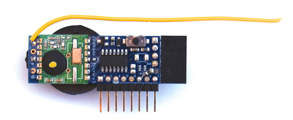
Software hell

In Software on Jul 6, 2010 at 00:01

I wish this were an exceptional tale. But it isn’t, it’s the norm…

I run a webserver for Jee Labs and a couple of other web sites and services.

Screen Shot 2010 07 02 at 23.55.19

I wanted to add support for logging the last hours of a new “#jeelabs” IRC channel. IRC might not be a good fit for me personally, but since several people have asked for it, I do want to support it. With say the last 3 days of that discussion logged as some public web-pages, I could drop by once in a while and try and add to the discussion going on at that time.

The “eggbot” system was suggested to me as a way to accomplish this:

Screen Shot 2010 07 02 at 23.55.50

Ok. Server is Debian, so “aptitude install eggdrop” should work, right? Debian is good at package management.

Wrong.

Turns out my server is still running Debian Etch, and “Etch is end-of-lifed”, as I just found out. The server ISP’s repository is gone. No updates, no installs, no security fixes, nothing.

Ok. Better upgrade Debian Etch to Debian Lenny first.

I’ve been there before, I know how to do it. Takes a few hours, but then it’s done. Server is running Lenny now, and all the main servers and services are still running fine (impressive!). This is a server in Germany, btw.

That was yesterday (well, ehm… night).

Today, quick check. Server ok. Weblog ok. Forum ok. Cool.

Oops. Ikiwiki isn’t working anymore. That’s the software I use to convert the Markdown pages into the Cafe web site. Fully scripted, based on Perl.

Ikiwiki wasn’t installed as Debian package, because the one in Debian was waaaay too old. Even on Lenny, it lags (by over a year – Debian Lenny still has 2.x, Ikiwiki has been at 3.x for some time now).

Ok, so let’s try to re-install it from source. By now, usually all my warning systems go into in high alert mode, because source installs are a different ball game (even with a “scripted” language such as Perl, how ironic!).

The Ikiwiki installation page is reassuringly short. Three steps. First two look pretty easy, right?

PERL5LIB=`pwd` PERL_MM_USE_DEFAULT=1 perl -MCPAN \
    -e 'CPAN::Shell->install("Bundle::IkiWiki")'
PERL5LIB=`pwd` PERL_MM_USE_DEFAULT=1 perl -MCPAN \
    -e 'CPAN::Shell->install("Bundle::IkiWiki::Extras")'

Wrong.

I’m now waiting for step 2 to complete.

More than 10,000 lines of text have scrolled over my terminal window so far. This sort of drivel:

Screen Shot 2010 07 03 at 00.05.40

More than two hours have passed.

More than 180 Mb of disk space has been consumed.

I’m forced to watch closely, because disk space is running low on the root partition. And this is running as superuser, so it’ll bring down the server if it fills up the disk.

Pinch me, am I really in the year 2010?

Screen Shot 2010 07 03 at 00.08.42

My complaint is not that some things are complex and require a lot of work and understanding.

My complaint is that some things are NOT complex and yet you get treated to an incredible amount of nonsense. Not to mention the fact that the problem isn’t solved until you invest in figuring out every detail of lots of different kinds of packages.

The IRC logging? Not solved yet. I can probably write a 200 line script with not a single dependency on other code which does what I need: track the last 100 hours of an IRC channel disscussion as a web page.

The Ikiwiki setup for the Jee Labs Cafe? Broken. One week of work to write a Markdown parser and generate the static pages myself, would be my estimate. Probably well under 1000 lines of code, all in a single script. Three orders of magnitude less disk space, and easier to adjust to my needs.

I’m still waiting for the second step of the Perl install to complete. It’s running a “BigInt” package without proper library support, apparently. Falling back to “Math::BigInt::FastCalc”, and running tests which take ages:

Screen Shot 2010 07 03 at 00.26.24

Could someone help me understand where a static wiki page generator needs to do cryptographically secure factorization of large primes or something?

I’m stumped. Three hours waiting now. I give up.

I’ve aborted the (non-) install. With 220 Mb disk space gone, and no clue how to get it back. Oh yes, wait, it’s all in “~/.cpan” of course – how obvious. Thank you, Ikiwiki & Perl, for breaking down. Thank you, Eggdrop, for making simple things hard. And thank you Debian Linux, for not giving me the option to go back to my previous setup.

And you know what ticks me off? All of the above can be avoided. It has been solved.

But we’re living in medieval times, clearly. Most people haven’t even heard of Starkits. What a cruel joke.

Ah, wait. Maybe I’m the only one who runs into issues like these. Maybe everyone else has servers which just work, and to which you can add functionality without getting stuck. Doing everything you want. And a breeze to upgrade, of course.

That must be it. It’s just me. I have totally unrealistic expectations.

Apologies for the rant. Normal transmissions will resume tomorrow…

Update – thanks to a backport tip in the comments, Ikiwiki is now working again.

Uploading? ISP? FTDI? Huh?

In AVR, Hardware, Software on Jul 4, 2010 at 00:01

There seems to be a fair bit of confusion in- and outside the Arduino world, and it’s spilling over to JeeNodes …

I’d like to go through some terms and buzzwords to try and clarify how to get your Arduino or JeeNode to do the thing you want it to do. I’m going to assume that you are familiar with the process of writing software (“code”), compiling it, and running it – at least on a Windows, Mac, or Linux computer (let’s call them all PC’s for now). With software for the ATmega, there are two approaches, depending on whether you use the Arduino IDE or not:

Screen Shot 2010 06 28 at 23.50.22

Both lead to the same result: a “hex” file with code that needs to be transferred from the PC to the ATmega.

The step which can be puzzling when starting out with physical computing and embedded hardware is how to get things across from your PC to that little Arduino or Arduino-like system you’re holding in your hand. And vice versa, since we often want to get results back or see some confirmation that things are working properly.

The confusion comes from the different conceptual levels involved, and things like:

  • do you mean how to connnect? – plug in a USB cable
  • do you mean how does the ATmega change its own code? – through a boot loader
  • do you mean via ISP (In System Programming)? – no, that’s normally not needed
  • do you mean via FTDI? – yes, that’s the name of the chip which is hooked up to USB
  • isn’t FTDI a connector? – yeah, that too, sort of… i.e. a 6-pin convention
  • isn’t a power + serial cable enough? – no, resets also play a key role
  • do I have to use the Arduino IDE? – no, you can also use a program called “avrdude”
  • what’s avrdude? – a program which can upload to a boot loader or an ISP programmer
  • do I need an ISP progranmmer? – nope, the boot loader does essentially the same thing
  • so why not just get rid of ISP? – because you need ISP to install the boot loader

Confused? Welcome to the club…

In case you’re wondering… the process is called “uploading” because the PC initiates this as outbound transfer:

Screen Shot 2010 06 29 at 01.51.50

To get your code (“sketch” in Arduino-speak) into an ATmega, you need three things, working together to make uploading happen under all possible conditions:

  1. An electrical connection – to power the ATmega, to communicate with it, and to restart the ATmega when it is stuck or busy doing something else.

  2. A common language / protocol – the communication must be understood by both sides, i.e. PC and ATmega.

  3. Software on both sides of the connection – Sending something when the other side isn’t listening, or listening while no-one is sending will not have the desired outcome.

Let’s go through each of these separately.

1. An electrical connection

There are several ways to make the connection. With an Arduino, or any similar board which has a USB connector, you can simply plug in the USB cable:

Screen Shot 2010 06 28 at 23.52.41

Some boards use a separate USB interface (“FTDI adapter”), allowing reuse of that interface for multiple boards:

Screen Shot 2010 06 28 at 23.54.08

The end effect is the same: a connection which powers the ATmega and allows communicating with it using a simple serial protocol. There’s also a trick in this hookup to let the PC reset the ATmega whenever it wants.

2. A common language / protocol

Ah, now it gets interesting. First thing to note is that there is no single common language / protocol!

That’s right. It all depends on what you want to do. Here we want to upload code from the PC to the ATmega. That requires exchanging “ISP commands” over the connection. But once uploading is done, we really want to reuse the connection as a regular two-way serial link.

The way it works is that the PC will reset the ATmega just before uploading new code. This activates a “boot loader” on the ATmega. Now both sides will be in sync (briefly) so they can exchange the necessary information to make an upload happen. IOW, right after reset the protocol is “ISP commands”. Once the upload is done, the connection can be reused for any protocol you like – as determined by the code that was uploaded.

3. Software on both sides of the connection

Back to the software now. We need to send ISP commands over the connection.

As you may have guessed, that’s exactly what the Arduino boot loader on the ATmega understands. When reset, the boot loader in the ATmega gets control. It waits and listens for incoming STK500 ISP commands. If none come in within a second or so, it relinquishes control to whatever was previously uploaded to the ATmega.

On the PC side, we need software which resets the ATmega and then immediately sends all the ISP commands needed to transfer and program the contents of a hex file.

This is what “avrdude” does. You can either use it implicitly from the Arduino IDE by starting an “Upload” from the menu, or you can launch it manually from the command line – avrdude needs a few options to tell it where the USB port is, what baudrate to use, the type of ATmega, the protocol to use (i.e. STK500), etc.

There’s more…

The above describes the different pieces and concepts involved in getting code into an ATmega. The beauty of it is that once it works, it really works well. Supplying power, uploading, communication, control, debugging … all with one simple USB cable. You only need to go back a few years to appreciate just how much this approach simplifies embedded development.

But there’s one important detail: the ATmega has to have a functioning boot loader. Placing a boot loader into an ATmega is a bit more complicated (and involves other things such as “fuses”). It’s a chicken-and-egg problem.

This is where the ISP programmer comes in. An ISP programmer is a fairly simple piece of hardware. In fact, you can make your own, as I’ve described in several posts on this weblog. See this and this post for some quick solutions which require nothing more than a working Arduino or JeeNode.

The good news, is that you usually don’t have to worry about installing the boot loader – it’s all done for you. Once. For the mechanism described above, you’ll never need an ISP programmer.

Some people actually prefer to use the ISP technique for uploading their sketches. In fact, sometimes you have no choice, i.e. when you need the serial port at all times, or when you can’t spare the 1..4 Kb required by the boot loader code, or when working with ATtiny chips which don’t support bootloaders.

In thoses cases, you’ll need a setup with an ISP programmer. But for most people doodling around with ATmega’s and the Arduino IDE, the above boot loader mechanism is usually very convenient and the easiest to get going.

Either way, it helps to understand the process. I hope the above was helpful in that direction.

Fixing a faulty ATmega (Arduino)

In AVR, Hardware, Software on Jul 2, 2010 at 00:01

After a recent post on how to repair an ATmega with a faulty (or even missing) bootloader and helping someone out with it, it occurred to me that this mechanism will work for any Arduino – not just JeeNodes.

Any 3.3V or 5V Arduino’ish system which lets you upload the isp_repair.pde sketch can be used to program any board with an ISP connector on it. The code is for ATmega328’s, because that’s all I use around here these days.

The trick is to hook up a few power and I/O lines in a specific way:

Screen Shot 2010 06 28 at 16.59.11

I’m using an Arduino Pro as example, but that’s just one of many you could use. Now connect these six wires:

  • ISP pin 1 = BLUE = Digital pin 4
  • ISP pin 2 = RED = VCC (+5V)
  • ISP pin 3 = GREEN = Analog pin 0
  • ISP pin 4 = PURPLE = Analog pin 3
  • ISP pin 5 = ORANGE = Digital pin 7
  • ISP pin 6 = BLACK = GND

Note: if your working board operates at 3.3V, then you should connect the RED wire to +3.3V, not +5V (that way signal levels and power supply will match). Also: the target board should not be connected to anything, since it will be powered through the ISP connector.

The only thing left to do is to upload the isp_repair.pde sketch to your working board, and open up a console window. You should see something like this:

That’s it – disconnect all the wires. The ATmega on the target board now has a boot loader and the standard pin 13 blink sketch. Ready again to accept whatever sketch you upload to it!

Uploading without avrdude

In AVR, Software on Jul 1, 2010 at 00:01

In the future, I’d like to upload new firmware to JeeNodes, Arduino’s, and other AVR boards through channels other than a serial port or USB. Uploading to a “slave plug” via I2C would be neat, for example.

That means the standard avrdude won’t do. Besides, after having coded various types of ISP sketches recently, I realized that the upload mechanism is really quite simple. If all you need is STK500 compatibility (as used by several ISP programmers and by the Arduino boot loader itself), then avrdude is overkill.

So here’s a demo “rig” for JeeMon which does the same thing as avrdude, i.e. upload a sketch over a serial port:

Screen Shot 2010 06 27 at 23.19.45

That removes the need to compile and install avrdude. Better still, this should work as is on every platform supported by JeeMon.

(Note: the above code is now part of JeeMon, but the source code can also be found here on the web)

Onwards!

Update – the above code has been integrated into JeeMon as new Upload rig – with dudeLoader renamed to “stk500” and readIntelHex now called “readHexFile”. Here’s a new demo “application.tcl” using this:

Screen Shot 2010 06 28 at 01.46.48

Now works with the Arduino boot loader as well as with the Flash Board ISP programmer (add “19200” arg).

(Reminder: the Jee Labs shop will be closed from July 14th through August 14th)

Going for gold with the BMP085

In Software on Jun 30, 2010 at 00:01

The recent post about adding some battery savings logic got a lot of mileage out of a very simple change – more than 10x lower average power consumption.

Warning: getting power consumption down can be an addictive puzzle!

Jörg Binkele was very helpful, and sent me a scope image, measuring the voltage drop over a 10 Ω resistor in the power line (before the regulator). Here are the first 5 seconds after powering up:

Jeenode Start tb0

As expected, the node settles into a very low power mode most of the time, with an occasional blip once a second. FYI: one vertical division is 10 mA. The little horizontal bar at both ends is probably the trigger level.

One small surprise was the startup behavior. Well, that first 18 mA bump is really a very simple bug: in the first second when the timer is running and being polled, the node is not in low-power mode. Aha, of course – my power-down logic is at the end of loop(). Ok, trivial to change – just move the end of loop() to the beginning:

Screen Shot 2010 06 24 at 11.11.51

Yup, that seems to get rid of the 1 second hump @ 18 mA. Great. I don’t have an explanation yet for the initial 1.5 seconds, but I suspect that the RF12 driver is waiting in rf12_initialize() – there is still some oddness with RFM12B initialization after power-up. Oh well – that’ll be for another day.

But now it gets interesting – I told you it’s addictive! – the image above shows that each blip is ≈ 75 msec @ 18 mA. That’s when both the ATmega and the RFM12B are turned on.

Wait a minute. Why so long? Sure, the BMP085 needs to measure temperature and pressure, and that takes several tens of milliseconds. But why keep everything else running full throttle? There’s no need.

So I rearranged the core loop a bit, in a way where all major delays would be done with as much of the node’s hardware turned off as possible (bmp085demo.pde):

Screen Shot 2010 06 24 at 19.06.55

Here is the result, again courtesy of Jörg – and then annotated:

Detail Power use

There’s lots of info here. Please note that the time scale is 25 times more detailed than the first scope image. The fun part is that you can essentially tie each power level to a line of code.

For example, the first hump is when the timer hasn’t yet reached 1000 milliseconds (since the watchdog can only take steps of at least 16 ms), so the node waits. But since it uses idle mode i.s.o. normal mode, power levels are about half of what an ATmega usually consumes. With almost no effect on the code. All we’re doing is switch off to wait for the next timer interrupt – that’s 50% of easily obtained savings.

Then there are two medium peaks when the ATmega starts the BMP085 measurements, and in between it drops back to power-down levels. Then we waste some power sending results out on the serial port (this could be removed). Lastly, when it’s time to transmit the readings, we switch on the radio, make sure it gets its job done, and then loop, again in power-down mode with the watchdog to keep us going.

If you look very closely, you can even see how long the BMP085 is busy with measuring temperature (about 4ms) and pressure (roughly 20 ms). Exactly according to specs.

The blip on the first screen is about 4 divisions on the second screen, and as you can see, the node is now asleep most of that time. That’s probably another 10-fold improvement. I wouldn’t be surprised if this node will now run a year or so on one set of AA batteries. And it’s still reporting once a second.

The moral is: match your reasoning to measured facts, and you can get a lot of power savings. Each case will be different, but it’s not rocket science.

Thanks Jörg, but please don’t send any more scope shots … I need to kick this addiction again! ;)

(Reminder: last day of the June special in the shop!)

TwitLEDs finale

In AVR, Hardware, Software on Jun 29, 2010 at 00:01

The TwitLEDs project by Myra and Jean-Claude Wippler (daughter and father) has come to a conclusion. It was great. I’ll just summarize by pointing to the six posts on the Jee Labs weblog describing the technical details, and some pictures and videos, showing the results.

Here you can see the finished TwitLEDs robot:

Dsc 1741

This is the, ehm… print head?

Dsc 1749

And last but not least, some videos. First a trial run for the print mechanism:

Next, a trial run for the vehicle, trying to stay out of trouble:

And here the result!

And one more:

Ok, that’s it. Myra and I both had oodles of fun building this and trying things out – hope you did too :)

Onwards!

(If you can’t view the videos on vimeo, see 1, 2, 3, and 4)

RFM12B as spectrum analyzer

In Software on Jun 27, 2010 at 00:01

Intrigued by a very interesting post by “loomi” on the discussion forum, I wanted to find out more…

What he did was use the RFM12B as a crude spectrum analyzer: sweep the frequency across its entire range, and use the RSSI threshold and status bit to find out whether there is any signal on that frequency.

First of all, I added an rf12_control() function to the RF12 library, to allow access to the low-level registers of the RFM12B. This allows changing the frequency and RSSI settings, and reading out the RSSI status bit.

On the software side, a sketch is needed for the JeeNode which does the sweeping and measuring:

Screen Shot 2010 06 21 at 00.26.21

This reports one line of 476 digits 0..6 for each sweep. Each digit in this line of text represents the measured signal strength at that particular frequency.

The RSSI readout is very crude. All you can do is set a threshold and read out a single bit in the status register, telling you whether the signal is above or below the threshold. Tedious, but doable.

The fun part starts once you get to plotting this as a graph. I used JeeMon and wrote a Tcl/Tk script for it:

Screen Shot 2010 06 21 at 00.30.15

And here’s some sample output:

Screen Shot 2010 06 21 at 00.21.30

The green line is the default frequency setting of the RF12 driver.

Each sweep will add a set of black dots to the graph, but since the values are being accumulated in a “counts” array, the dots will creep higher and higher, drawing a bar as more sweeps come in. Using the current delays, one sweep takes a few seconds, so to get the above graph I had to keep JeeMon running for a few minutes.

When left running for some 15 minutes, the large bars will move out of range, but the smaller accumulated counts will now become clearer:

Screen Shot 2010 06 21 at 00.30.53

I haven’t figured out whether these values are valid, nor what could be causing all this RF activity. The peaks are fairly sharp though, so it would seem like a reasonable set of measurements.

TwitLEDs robot – action shots

In AVR, Hardware, Software on Jun 25, 2010 at 00:01

As promised in the previous post, some pictures and movies of the TwitLEDs robot in action.

First another view of the robot, with the different pieces:

Dsc 1747

We don’t have the proper “arena” yet, i.e. a big fenced-off floor area covered with glow-in-the-dark paint. Instead, these first trials used two pieces of foam board, taped together. It’s not perfect because the robot keeps running off track, and because the hump between the two pieces is quite high. Foam board isn’t really suited for this: it curls up too much from the moisture in the paint. We probably should have waited a bit longer for everything to dry completely…

The inital test code just printed out its name (povGlow) and the compilation date. In the first tests, one of the LEDs wasn’t working (a software bug, not hardware), so the text isn’t quite right:

Dsc 2039

You can clearly see the fading of the letters over time. This happens very quickly, but those faded letters then remain visible for quite a while. That’s why you can still see several trial runs “printed out” on the foam board.

So the basic idea of printing with light works, as you can see!

Here is a video (sorry, not inline), showing how the robot veers to the right as I put my hand in front of it to prevent it from running off the track. Note that I’m not touching the robot, I just briefly trigger the distance sensor. The on-board LED lights up in red when the correction takes place. It’s not very smooth, but it works.

Another picture, showing the decay of the printed text brightness:

Dsc 2067

Maybe 7 pulsed blue lasers (from DVD writers, perhaps?) could be used to create even more intense blue dots. As it is, with these blue LEDs the writing is very clear – but only in a relatively dark room. With the lights on, the text becomes virtually invisible. Even though the LEDs are bright enough to be painful to look at:

Dsc 1749

The quality of this “printer” is actually pretty good, considering how simple its technology is:

Dsc 2056

Finally, a run where the robot happened to stay a bit longer on track, allowing it to display its brief message a few times. Again as video – you can see the wobbling foam board, and this thing driving like a drunken duck, leaving its trail of fading messages behind.

All that remains, is to try and get some tweets into it in real time. Stay tuned…

Several days of testing have now drained the 4 alkaline AA to the point where the robot advances noticeably slower. Looks like we’re getting no more than an hour or two out of these batteries. Which is not really surprising: the DC motors must be eating quite a bit of current, and the LEDs probably draw up to 200 milliamps or so. Self-powered autonomous motion is really hard!

TwitLEDs robot, part 3

In AVR, Hardware, Software on Jun 24, 2010 at 00:01

To continue on yesterday’s post, here is how we got a little autonomous robot going.

The main part was solved by picking the Asuro robot kit. It’s really low-end, but it has just enough functionality for this project, and at €50, it’s very affordable. In fact, Myra built a spare one because the first unit broke down. In the end, I was still able to fix it: a burnt out transistor (both H-bridges are done with discrete components!). So now we have two Asuro’s:

Dsc 1750

The nice bit about the Asuro is that it has an odometer on each wheel. IOW, there are IR LEDs + sensors to count the number of steps (8 per rev) made by the wheel, and the C library code includes logic to adjust the speed of the motor. It’s a bit crude, but because of this the Asuro can drive fairly straight. As we found out later, it has a bit more trouble doing so while driving slowly, so it’s still a bit wiggly.

But it works. Two small DC motors, some simple gears, motor axles soldered to the PCB (what a great low-cost solution), and room for an extension board. To give you an idea of how crude this thing really is: there is no on-board voltage regulator. When used with 4 alkaline AA batteries, you have to remove a jumper so the extra voltage drop over a diode gets the supply voltage down to under 5.5V …

The Asuro is full of such nifty cost-cutting tricks. It even includes a bidirectional IR link, over which new code can be uploaded. The IR link is very short-range, so it would have been insufficient for our purposes – but for quick code tweaks, the IR link works fine.

Speaking of code, here is the main avoider.c logic running on the ATmega8:

Screen Shot 2010 06 18 at 23.57.08

This is not an Arduino sketch, but I made it look a bit like one by using the same setup() and loop() functions.

This code has to be compiled with avr-gcc. The Asuro comes with several examples with Makefiles. I simply copied one and started extending it. A little optional USB-IR adapter is used to connect to the Asuro (an RS232 one is included with the Asuro kit, but I don’t have any RS232 ports). The whole setup works pretty well from the command line, especially considering that it’s a completely different setup than the Arduino IDE.

Anyway, back to the design of the TwitLEDs robot.

The challenge was to find a simple way to make this robot drive around without bumping into things. The Asuro has a row of switches at the front, but these are not very reliable, and besides: bumping and stopping and turning would mess up the LED strip being “printed” on the glow-in-the-dark paint.

So instead, we mounted a Sharp 10..80 cm distance sensor on top. It’s very easy to read out, since it produces an analog voltage, inversely related to the distance of objects in front of it.

The logic for collision avoidance is crude, but sufficiently effective: turn more and more right as you get nearer to an obstacle. The on-board LED turns from off to green to yellow to red as the distance decreases, so it’s easy to see what the robot is doing. I’ve tweaked it so that when it drives straight towards an obstacle, then turning will be quick enough to never bump into that obstacle.

Here’s the completed unit, with the Sharp proximity sensor on a little expansion board at the front, and the LED blinker glued to the side of the battery pack – the LEDs hover 1 .. 2 mm above the ground:

Dsc 1741

Myra’s idea was to have this thing drive inside a more or less circular “fence” made of corrugated cardboard. The whole area inside the fence will be made of some panels, covered with 3 layers of glow-in-the-dark paint.

There is a flaw in the current design, in that the robot can only evade an obstacle by turning to the right. If it approaches a wall obliquely from the right, it will do the wrong thing and drive straight into the wall. But we’re hoping that as long as it doesn’t over-correct, and by sending it off in a tangent, it will keep adjusting slightly to the right as it drives around and around in “sort of” circles.

More tests and tweaks will no doubt be needed.

But as it is, this thing really seems to stay out of trouble. We can let it loose in the room and it’ll veer to the right whenever it comes near an obstacle. Sometimes it veers to far, though. Again, I hope a more controlled “arena” will be sufficiently simple to keep it going.

When the robot does bump into its front switches, it turns both motors off, blinks for 10 seconds, and then starts off again. Time enough to pick it up and aim it in a different direction.

So that’s it. An autonomous unit with two independent computers, IR distance sensing, a short range IR link, and the JeeNode with a longer-range wireless RF link. Even including a JeeLink on the laptop side, the cost of all this was only slightly over €100.

Tomorrow, some pictures + movies. Gives me time to finish the Twitter link, and then on to the grand finale!

(Reminder: one week left for the June special in the Jee Labs shop!)

TwitLEDs robot, part 2

In AVR, Hardware, Software on Jun 23, 2010 at 00:01

Yesterday’s post introduced the robot Myra and I have been working on. Here’s the first part we built:

Dsc 1725

It’s basically a backplane for the LED blinker component. Or to put it differently: a simple persistence-of-vision (POV) unit, using a JeeNode, and Output Plug to drive a few LEDs. Only the output plug was soldered-in permanently. The removable JeeNode allows it to be easily programmed and re-used, and the removable LEDs allow trying out different units. This turned out to be important, because I only had a few green LEDs when starting this, and had no idea then as to what sort of LEDs would give the best POV results later on.

Myra did all the soldering. Here are the two LED mounts we ended up with:

Dsc 1745

The one on the left is the super-duper LED concoction we built as final version. The one on the right was great for initial testing.

Everything is held together with rubber bands, zip-lock ties, tape, and ample amounts of hot glue (once verified to work!) – hacking at its best, clearly:

Dsc 1742

Here’s the LED blinker with the final LED strip, side view:

Dsc 1743

Side view close-up – with the foam board cover:

Dsc 1746

Bottom view:

Dsc 1744

Seven blue LEDs, ready to shine very brightly and controlled by the JeeNode.

The software started out very simple, of course. Things like this, just to make sure it all works:

Screen Shot 2010 06 18 at 23.01.21

This is the main part of what is more or less the final twitLEDs.pde sketch:

Screen Shot 2010 06 18 at 23.03.06

I found a suitable font table by googling around a bit. This is needed to go from ASCII characters to dots-in-a-readable-pattern. No room for Unicode (don’t laugh: some tweets are in Japanese and Chinese, and they won’t show properly).

The amazing bit is that everything worked essentially on first go. It blinked! But does it blink in the proper pattern? Our first test consisted of Myra taking a long-exposure shot, as I waved this thing around in the air – with the lights off. Liesbeth tracked progress through all the shrieks and laughs… but from a safe distance :)

Dsc 1793

Yippie. It really works!

Tomorrow: driving around without bumping into things.

Something different…

In AVR, Hardware, Software on Jun 22, 2010 at 00:01

Ok, so I’ve got tons of projects on my plate to do and to finish. And tons more that are still very experimental, or haven’t even been started. Plenty to keep me busy, with the summer vacation period nearing fast.

Yet here’s something different. The timeline for this project was imposed by external factors: my daughter Myra doing a project for the last quarter of her second year at the Design Academy in Eindhoven.

She wanted to do something which triggers human interaction, and she wanted to try something with Physical Computing. “Terrific, I’ll help!” – I shouted, completely ignoring all the pending work on my own plate…

So here’s the start of a few articles about the “TwitLEDs” project we’ve been working on recently. All the basic ingredients work as I write this, but we have yet to finish the final setup and go through a last rehearsal.

What is it?

It’s a mix between a matrix printer and a persistence-of-vision (POV) display.
It’s called the TwitLEDs robot. And it’s hooked up to the internet.

Get it? No? Ok, then let me try again. I think this picture tells it best:

Dsc 2069

The idea is to have a little autonomous robot driving around, leaving messages behind on a floor covered with glow-in-the-dark paint. The messages are collected off Twitter using a configurable search term. This is done from a laptop and then sent to the robot by wireless.

There were several fairly non-trivial problems to solve here, with some experimentation needed to find a workable mix – as well as some time contraints. A few days of work would be the most I could set aside for this. Luckily, I didn’t get lost in too many dead alleys, so it worked out nicely.

Here are the pieces we used:

  • A low-cost robot kit called Asuro – based on an ATmega8, so I had all the software ready for it. In fact, I played around a bit with it a while back – as reported here.
  • A JeeNode for wireless connectivity.
  • An Output Plug to drive some LEDs.
  • Seven blue LEDs. I picked a bright one with a very focused beam (C503B-BAN-CY0C0461).
  • Glow-in-the-dark paint. Green stuff. Three coatings.
  • Some panels to create a floor. Covered with the green stuff.
  • Some cardboard to create an “arena” on the floor to contain the robot.
  • JeeMon running on a MacBook, with a JeeLink to send out the messages.
  • A fairly dark room. This just won’t work with the lights on, unfortunately.

As with every project, the first part is the hardest and the most critical success-factor: figuring out what to do, what not to do, and finding solutions within the many constraints we had to operate under. I’ll spare you the ideas that didn’t make it, and the (really neat) ideas we simply didn’t have time for.

Being the sole programmer on the team, I got to deal with all the software. Yummie! :)

The most important insight for me was that we could implement this project with three completely independent subsystems:

  • The LED blinker, driving 7 LEDs in the proper pattern, basically a POV unit (plus receiver).
  • The robot, moving around while continuously trying to stay out of trouble.
  • The server process running on the laptop, connecting to Twitter and sending messages into the air.

We started off with the LED blinker because it was a major component with few unknowns, i.e. we picked the low-hanging fruit first. Here’s a picture of it, still under construction:

Dsc 1726

More on the LED blinker tomorrow…

A small improvement to rf12_sendStart()

In Software on Jun 21, 2010 at 00:01

The RF12 driver has a function called rf12_sendStart() which – you guessed it – is used to start sending out a new wireless packet.

Yesterday’s post was about battery savings, which I implemented by going into a power-down state right after sending out a new data packet.

That code included this little detail:

Screen Shot 2010 06 20 at 03.50.41

The reason for this is that the RF12 driver works mostly on an interrupt basis – i.e. in the background. Without the delay, the node would power down before the packet had actually been sent out. Then, when waking up, the transmission would fail due to the transmitter underrun caused by this logic.

By simply waiting a bit, the interrupts can continue to take place, and all the bytes will get sent to the RFM12B and from there into the airwaves.

Totally by chance, an EtherCard software problem was reported on the Jee Labs discussion forum, which turns out to be related to this very same issue. Sure enough, adding the “delay(5);” fixed that problem as well.

This felt a bit unsatisfactory as solution, so I’ve extended the rf12_sendStart() function to support a “synchronous mode”. The change is backwards compatible, i.e. the default behavior of rf12_sendStart() hasn’t changed.

Now, if you pass 1 as fourth argument, rf12_sendStart() will wait for the packet transmission to actually complete before returning to its caller. In general, calling rf12_sendStart() in sync mode is probably a good idea. Sync mode can be used for sending data packets as well as acknowledgement packets.

So the above code can be replaced by this single line:

Screen Shot 2010 06 20 at 04.02.11

This simplifies the bmp085demo.pde sketch slightly, and it also solves the problem that the EtherCard library may occasionally lock out interrupts on the SPI bus a bit too long to keep the RF12 driver running.

The code and documentation have been updated.

Onwards!

Battery savings for the Pressure Plug

In AVR, Hardware, Software on Jun 20, 2010 at 00:01

Reducing power consumption is fairly tricky, as you can see in the many previous posts about this topic. And to be honest, I haven’t quite gotten to the point where I want to be with the Room Board. My first “major” (ahem) setup with about a dozen nodes around the house didn’t quite go as I had hoped. Most batteries were empty within a month. A few nodes are still going, but those are hooked up to power adapters…

I’d like to revisit this issue and try to improve things a bit. To make the rooms sketch perform better, and also to make the code structure a bit clearer. The current rooms code is quite complex and hard to follow.

But before messing with the rooms.pde sketch, let’s tackle something simpler: the wireless sensor node based on the Pressure Plug, as described here, and then simplified here. I’ll use that last version as starting point.

The first point to note is that to get a substantial first power reduction, you have to focus on the portion of the code where it’s spending most of the time. Which, in the case of “bmp085demo”, is here:

Screen Shot 2010 06 17 at 01.55.06

That’s right: it’s waiting for the next second to “happen”. And even with a slow’ish sensor such as the BMP085 at maximum resolution, it’s spending more than 90% of its time there… waiting!

I’ll use an approach which might be a bit surprising: let’s not change any of the current logic. The idea is that once we’ve done our thing for the current second, we can go into low power mode, as long as we make sure to get back to normal operating conditions in time for the next second.

So what we’re going to do is add some code to the end of the loop() function. It’s functionally equivalent to adding it at the start, since loop(), eh, loops – but I think it makes a better point.

The end of loop() used to look as follows:

Screen Shot 2010 06 17 at 02.01.01

I’m changing it to this:

Screen Shot 2010 06 17 at 01.43.00

IOW, at this stage all the hard work has been done. We wait a bit for all interrupt-driven I/O to complete (serial and RF12). And then we need to figure out how much time remains until the next second. The power saving happens by spending that time in power off mode.

But this requires some preparation. When inducing a comatose state like this, you have to make absolutely sure that something is still able to get you out of coma and back up and running again. This is what the ATmega’s “watchdog” is for: we set it up to wake us up in 16 milliseconds, just before entering sleep mode. And then we keep doing that until it’s almost time to take another reading. The actual watchdog interrupt handler does nothing, btw – all we want is to get back out of power down.

Note that the radio also needs to be turned off and back on again. It’s the biggest power consumer when enabled. Turning it off and going into power down mode is what lets us go from a tens-of-milliamps current drain to a tens-of-microamps current drain.

All the logic for this is located in the loseSomeTime() function, which was adapted from a slightly different version in the rooms.pde sketch:

Screen Shot 2010 06 17 at 01.42.33

And that’s about it. The average power consumption of this sensor node will go down by an order of magnitude. It’ll still be 1..2 mA, but it’s a major improvement: this node should now run 2..3 months on AA batteries. The source code for bmp085demo.pde has been updated.

I’d like to stress that such gains require very little effort for many types of sketches. All you have to do is figure out where the sketch is spending most of its time, and deal with just that part of the code. Getting into yet lower power consumption levels would require more work.

Input Plug, oh my

In Hardware, Software on Jun 19, 2010 at 00:01

More fallout from the bad ISP programmer. As reported on the forum, there is a problem with the Input Plug. Fortunately, it’s fixable in software.

The problem is that the ISP programming of the ATTiny45 chip on the Input Plug had the same problem as the recent, ehm, Murphy debácle: the fuses weren’t always set properly.

So the ATTiny starts up running at 1 MHz i.s.o. 8. And hence the timing is off when driving pulses to it to control the analog multiplexer.

The solution was to add a “fix” parameter to the InputPlug class in the Ports library. It defaults to 0 (no fix needed), but when set to non-zero, the timing is adjusted to slow down by a factor 8. That way, channel selection will take a bit longer – but at least it’ll work:

InputPlug myPlug (3, 1); // plug on port 3, slow down for wrong ATTiny fuse

This code has been added to the Ports library. There is a downside: the fix means that channel slection now takes roughly 900 µs, instead of the intended 100 µs.

Next question is: how to make sure this won’t happen again? – Answer: build a test jig, so all plugs can be tested fully before shipping. Trouble is, all Input Plugs ship as follows (this is an early hand-soldered unit):

Dsc 1732

Without headers!

My mistake was of course that I would wing it, and avoid the testing. Bzzzt. Time to build a little test contraption:

Dsc 1733

The other side is filled with 17 tiny 1 kΩ SMD resistors, creating a voltage divider with 16 different voltage levels. Soldering this was quite a challenge, btw:

Dsc 1737

And now I can take advantage of the fact that everything is gold-plated. So the following will make contact, just with the pins being pushed in and pressing lightly against the board:

Dsc 1735

I’ve been using the same trick for some time now, to test other plugs. Here’s how to connect the whole thing to one of the ports:

Dsc 1736

Below is a little readout test – a better test setup would be to simply perform the check and display a go / no go signal, but for now I’m just reporting the 16 values:

Screen Shot 2010 06 16 at 19.00.21

Sample output:

Screen Shot 2010 06 16 at 20.24.30

As you can see, the selection is now working reliably (once connected).

So that proves the bug and gives me a new tool to test Input Plugs before shipping. And of course I’ll re-flash the ATtiny45 chips on all remaining Input Plugs in stock at Jee Labs. For those already out there: you can either use the software fix, or send your Input Plug(s) back to me and I’ll fix the fuse settings to make selection snappier, as originally intended.

Problem solved. Phew.

Does it feel good to have to confess to another goof-up on my end? Of course not. But worse than that would be to keep quiet on this – and I won’t. I’m human, I make humiliating mistakes (LOTS!), I occasionally cut corners, but I do my best to learn and deal with it all. There is no doubt whatsoever in my mind that every person and company goes through these sorts of mishaps. It’s just usually not out in the open for everyone to see. Well, at Jee Labs, it doesn’t work that way – this is open source: software, hardware, goofs … e v e r y t h i n g !

A little GUI for the RGB LED strip

In Software on Jun 16, 2010 at 00:01

After yesterday’s post, this RGB strip control project is essentially done. Keep in mind that I’m doing this only to adjust what comes out as “white”. I’ll leave light levels and color variations up to nature, since all I need to do is look out the window…

But since wireless control is present anyway, I might as well create a little demo using the JeeMon software.

So here goes. The setup I’m using is as follows:

Screen Shot 2010 06 14 at 16.31.37

The JeeNode is configured as node 30 and the JeeLink as node 1 (in the same group). The manual way to send out a color command via serial USB is to type:

<red>,<green>,<blue>,<white>,30s

Where each of the four values are in the range 0..255 (0 = off, 255 = full on).

Now the GUI version (Mac OS X):

Screen Shot 2010 06 14 at 18.21.51

The code for this is as follows:

Screen Shot 2010 06 14 at 18.16.26

Like everything in JeeMon, it’s cross platform since it uses Tcl/Tk.

Here are the screen shots for Linux (Ubuntu) and Windows (W7, XP, 2K), respectively:

Screen Shot 2010 06 14 at 18.01.42 Screen Shot 2010 06 14 at 18.35.25

Screen Shot 2010 06 14 at 18.14.21 Screen Shot 2010 06 14 at 18.09.26

As you can see, the light gray background color was adjusted for the Mac – on some of the other platforms it needs to be darkened a bit to match the default label background.

Anyway. I’m not a GUI wizard, so this’ll have to do for now…

Remote RGB strip control

In Software on Jun 15, 2010 at 00:01

To continue this series on driving RGB strips with a JeeNode, here is a sketch which allows setting the brightness levels using PWM. It’s a bit long for a weblog post, but I thought it’d be useful, since there is quite a bit of trickery in here. Notes follow below:

Screen Shot 2010 06 11 at 23.17.29

This code does some hefty bit manipulation. The idea is to keep an array of 256 time “slots”, with bits to indicate when an I/O pin should be toggled on or off. The loop then continuously scans these slots at the rate of ≈ 32 microseconds per slot (this corresponds to roughly 120 Hz). The 8 bits in each slot map to the JeeNode’s I/O pins: bits 0..3 = AIO1 .. AIO4 and 4..7 = DIO1 .. DIO4.

A refinement is that only the first 255 of the 256 slots are scanned. This way, 0 is 100% off and 255 is 100% on.

The static “masks” array defines which setting gets mapped to which I/O pin. It depends on the way the output driver is connected to the JeeNode.

The main PWM timing loop is done fully in software. It will run slightly irregularly due to timer interrupts and RF12 driver interrupts, but the effects aren’t noticeable.

The RGBW values are stored in EEPROM, so that the LEDs come back on with the same settings after power cycling. The settings can be adjusted by sending a packet with the new values to node 30, group 5 @ 868 MHz.

This sketch could be extended to support “animations”, i.e. ramping up/down to specific levels, mood lights, etc – I’m not interested in that, I just want to be able to trim the color of my room lighting to a pleasant level of white:

Dsc 1723

All I did to adjust the strip on the right was send the following “RGBW” command out via a JeeLink:

255,140,40,120,30s

The above sketch does PWM, but this whole thing is still being turned on and off with an old-fashioned mechanical switch … if you still remember those :)

FWIW, I’m considering making a dual-channel “MOSFET Plug” – two of those could then be used to replicate this same setup for the LED strip on the left.

Tomorrow: a little GUI front end for all this.

RGB driver board

In Hardware, Software on Jun 14, 2010 at 00:01

To follow up on yesterday’s post, I made a more permanent 4-channel board for driving an RGB LED strip plus the original white LED strip already in use.

A JeeNode is used to drive these strips, using a small custom JeePlug to hook up ports 1 and 4, as well as to use the LED voltage as power source for the JeeNode:

Dsc 1717

Here is the plug in more detail:

Dsc 1718

It includes an LP2950 linear regulator to put 5V on the PWR pin, that way this thing can be used with any input voltage from 12 to 24V. Here is the bottom side:

Dsc 1719

The driver itself uses four IRLZ34N MOSFETs, three of which will be used for the RGB strip, and the other for the white strip so that it too can be controlled and even dimmed remotely:

Dsc 1715

The back side is hand-wired using sturdy copper wire, although in this case only 300 .. 600 mA is being switched per color. The 10 kΩ pull-down resistors prevent the lights from turning on in the absence of control signals.

Dsc 1716

And here’s the completed setup:

Dsc 1714

The two wires sticking out are for attaching my 12V lab power supply during testing. The other green 2-pin screw terminal is for attaching the white LED strip.

The RGB ledstrips can now be installed next to the LED strips already in use here at Jee Labs:

Dsc 1722

Here’s a trivial test sketch to turn each of the 4 colors on and off:

Screen Shot 2010 06 11 at 13.17.35

The results can be seen in this brief video.

What remains, is to write the software so this thing can be controlled via wireless. I might add an LDR to sense ambient light levels, or even a Room Board. Perhaps some basic ramp-up / ramp-down PWM logic. Or maybe I’ll just duplicate this setup and drive the two sets of LED strips I have, independently and from a single JeeNode.

Hardware is easy, it’s always the software… the code will be presented tomorrow!

Reminders: 1) June discount and 2) Jee Labs will be closed from July 14th to August 14th.

Driving an RGB strip with MOSFETs

In Hardware, Software on Jun 13, 2010 at 00:01

Another day, another project started. I have a nice 5-meter LED strip in the office, which provides indirect lighting at Jee Labs. Works fine, but despite being called “warm white”, it’s slightly greenish. Not so great…

Someone suggested adding an RGB strip next to it, to compensate for the color.

So to start off this multi-part series, I wanted to simply control RGB. This is very easy to do with three MOSFETs. I used IRLZ34N’s N-channel, since the LED strips are common anode. The circuit is trivial: source to ground, drain to LED cathode, and gate to an I/O pin. Rinse and repeat three times. I didn’t even add a pull-down resistor to the gate, though I probably should.

Here’s the circuit, fully connected to a test strip with 9 RGB LEDs using a separate 12V power supply:

Dsc 1664

I wrote a little test sketch which ramps the light levels up and down using PWM, and which goes through all the RGB combinations – using some bit fiddling:

Screen Shot 2010 06 07 at 13.17.10

The LEDs are pulsed in software, with a cycle time of 8160 µsec (32 * 255), i.e. roughly 120 Hz. No discernible flickering. A more advanced version ought to use interrupts to keep the PWM going in the background.

Here’s a video of the result – with apologies for the very low quality.

Since the JeeNode has RF on board, it will only be a small step to add wireless control. Stay tuned…

Update – Source and drain were listed the wrong way around, I’ve updated the text above.

IR trigger for Nikon camera

In AVR, Hardware, Software on Jun 12, 2010 at 00:01

Here’s a fun project: sending out infrared remote codes to takes snapshots :)

This is the code:

Screen Shot 2010 06 10 at 17.19.44

This sketch is doing everything in software, and it’s sort of pushing the limits by pulsing a TSKS5400S IR emitter LED at 38.4 KHz using software delay loops.

The timing diagram on this website was a great help to get this working in no time. Here’s another site.

With the 33 Ω resistor in series, total current through the IR LED should be somewhere between 20 and 50 mA. Since the latter is beyond the ATmega’s current sourcing capapbility, I suspect that the pin voltage will actually drop quite a bit below VCC. A transistor or MOSFET could be added for more power. As it is, this seems to trigger reliably up to about a meter away.

Here’s the setup, triggering my trusty D40 Nikon:

Dsc 1692

a self-portrait!

Lot’s of people have already done this ages ago, btw. Here’s a sketch which uses assembler to get the timing more accurate. But the above does work – the main point is to avoid digitalWrite(), which is relatively slow.

Long term decisions

In Software on Jun 11, 2010 at 00:01

This post is a question, but maybe I’m already answering it by posing the question in the first place …

The question is: what to do with the Jee Labs source code?

As you may remember, I went through a few mad gyrations recently w.r.t. setting up a community site using TikiWiki, and then quickly abandoning it again.

In the end, I’m glad I didn’t buy into TikiWiki. Too many compromises, and for my particular needs, far fewer benefits than I had originally hoped to see.

The current Jee Labs Café that has replaced it is very crude, visually, because I haven’t yet done the work to bring over the layout and style sheets from this weblog. But far more importantly, IMO, is that the information is finally organized in a sensible way – until someone tells me otherwise, anyway!

Screen Shot 2010 05 24 at 21.03.33

The pages are maintained by subversion (svn), a version control system which is well-known and widely used by software developers (as are the older “cvs” and the newer “git”), although I do find that a surprising number of people are not used to the whole idea of “source code control systems” and “code repositories”. Frankly, I couldn’t live without something like svn anymore, these days. It’s the only way to develop software and not lose your mind w.r.t. change management and long term maintenance – IMO.

Maybe I should go into the features and benefits of such an approach in another post.

My point here is that the entire Café website is managed by svn. This means that all older versions of pages, sources, documents, pictures, etc. are available. At least as importantly in this context, is that the pages can be edited by anyone with write access to the repository. It’s pretty simple: get a copy (“check out”) of the website, make changes, and write it back to the repository (“check in”). Writing is only allowed to those with a user name and password in the repository, so this is wiki-like, but not publicly writeable.

The interesting tidbit about the Café website is that all changes are automatically published on the web. I’m using ikiwiki as tool to take care of all that. Thats why all the pages for the Café can be maintained as simple Markdown text pages, and how the result ends up as HTML, with links and embedded images. I’m only using a very small subset of ikiwiki’s features, btw.

Another great side-effect of using ikiwiki is that the entire Café website consists of static web pages. No server load, inifinite scalability for free.

In practice, it’s all working out really well. I can easily update, extend, and maintain the Café website this way. And if anyone wants to participate and contribute more content for the wiki (one can always hope, eh?) then that would be very easy to fit in, since subversion can be used over the internet.

As far as I’m concerned, the daily weblog and the Café / wiki are in good shape for a long time to come.

There are two other areas. One is the Talk discussion forum, which uses bbPress. I’m not terribly excited by its functionality, nor by its (lack of) progress, but it’s holding out fine, sooo… if it ain’t broken, don’t fix it.

The fourth area of public Jee Labs activity is the source code being developed for use with JeeNodes and JeeMon. It’s been in my subversion repository for a while, then I moved it to Google Code, en then I moved it back to my subversion repository again, which is where it has been for many months now.

As fas as the repository goes, this way of managing source code works well, at least for me. But there are some sharp edges. For one, the web-browsing interface is based on ViewVC – which is a bit quirky, and which turns out to be CPU resource hog on my server. Probably just web-crawlers, constantly triggering CGI execution of the ViewVC Python scripts.

Also, I currently have no issue tracking system in place. Would be nice to get something going one day.

I’ve been looking into GitHub, which seems to attract a lot of attention (and open source projects), these days. It has git-based code repositories, with an optional svn interface, and it offers a wiki, issue tracker, and download area. Reminds me a bit of SourceForge, which seems to have fallen out of grace, these days.

My main concern with GitHub is that it’s yet another big central site, offering a mix of features and functions to attract as many developers as it can, with no guarantees that it won’t be gone a few years from now, or start doing “targeted” ads, or selling email addresses, or other nasty stuff.

There is, however, one tempting option out there: GitHub + JekyllJekyll is similar to ikiwiki, in that it takes text files (including Markdown, yeay!) and generates a website from it. Jekyll even offers a migration path for WordPress sites. The interesting bit is that GitHub supports Jekyll out of the box, and that it can be set up to work with custom DNS domains. IOW, I could merge this daily weblog, the Café, and the code repository into a single consistent system. The result could be one or two static websites (hm, I guess that rules out blog comments), fully under version control, and using the Markdown format I’ve already standardized on. Needs more thought!

As it currently stands, I think I’m going to stick with WordPress + subversion, which is rock solid and has some really nice software tools for it (like Versions on the Mac). Maybe just integrate the source code areas with the Café, and use ikiwiki to allow browsing the latest version on the web, right next to the supporting doocumentation.

It feels a bit like “going it alone” by placing everything in my own subversion repository and maintaining it all on a privately managed server, but all I can say is that a lot of what I’ve done in the past has been around a lot longer – and still is! – than some of those fads…

The web is somewhat too ephemeral for my tastes…

A Happy Ending!

In AVR, Hardware, Software on Jun 10, 2010 at 00:01

The multi-ISP programmer I built and started using some two weeks ago, turned out to be quite a nightmare. Not only were incorrectly programmed ATmegas sent out to about two dozen people, I also had to go through about 70 kits, prepared as new stock just days after I started using this programmer. Twice!

Yes, twice. Because the first “fix” turned out to be insufficient. Doh.

This was a clear case of one bug hiding another, and another, and another. Yep, four bugs: a bug in the MemoryStream class in the Ports library, a timing problem exposed by fixing that bug, and two incorrect assumptions about how the “avrdude” utility works. I’ve now got an explanation for everything that went wrong.

There’s no doubt some interesting psychology at work here … I was so proud of my idea op programming multiple ATmega’s! The main idea was to create an AVRISP-compatible unit which stores everything sent through it and then just replays the saved stream as often as needed. Trouble is, I jumped to conclusions the minute a first “run” worked. Roll the presses! Print it! Tell it to the world!

Anyway. There is a happy ending to all this!

The latest version of the isp_capture.pde sketch in the Ports library has been working properly for over a week now, programming well over a hundred ATmega’s (and it now does auto shut-down a few minutes after use):

Isp Capture Output

The last bug was a very puzzling one: everything worked, but sometimes the fuses wouldn’t get programmed. It turns out that avrdude first reads the fuses, and only sends out commands to program them if the fuses don’t match the new value. Since the programmer needs to work with brand-new as well as previously-programmed chips, the replay mechanism would have depended on the prior state of the chips: not good.

The solution is very simple: I now always program each fuse twice, with two different (valid) values. The second one will remain in force, evidently. Since the replay code was already ignoring fuse mismatch checks, this now means that even if the first setting is skipped by avrdude, the second will always be emitted.

Here is the shell script to prepare the Flash Boards:

Screen Shot 2010 05 30 at 01.35.40

So this has now become a very useful tool at Jee Labs:

Dsc 1432

I love the on-board LiPo battery: I can grab it, use it where I need it, and put it back – no wires = freedom!

For pre-loading the fuses, boot loader, and RF12demo, it already saved me a huge amount of time. Its “burn rate” is up to 500 chips/hour. And Mr. Murphy taught me some valuable lessons along the way…

And now it’s time to move on!

Repairing a faulty ATmega

In AVR, Hardware, Software on Jun 9, 2010 at 00:01

This post is being written after a pretty nasty foul-up on my part w.r.t. sending out badly-flashed ATmega chips. It’s probably too late to be of use to anyone involved in that little débâcle, but I thought I’d describe a DIY fix here in full detail anyway. I’ve simplified the code to make it even easier to use than what was described here.

So what is this about, eh?

The ATmega328 chip used in JeeNodes (and Arduino’s, and various other similar board) comes with a serial boot loader pre-loaded into the high end of its flash memory. This is arguably one the most important features that made the Arduino popular: it lets you upload a new “sketch” into the ATmega over the serial or USB port.

Lots of little details, but the point here is that the boot loader itself can’t easily be damaged, even if you load a non-functional sketch into the ATmega. Just resetting it will let the boot loader overwrite the flash memory with a new version – hopefully a better one. Basically, no matter what goes wrong, there’s always the boot loader in the ATmega to upload a new sketch to it.

There’s a chicken-and-egg problem, though: how do you get that boot loader into the ATmega in the first place? Well … you don’t. It’s normally placed there by the supplier of your ATmegas.

Since Jee Labs is one of the suppliers of JeeNodes (for Europe, and Modern Device for the US), I do need to do a little more. I use an “ISP” programmer to place that boot loader there, along with the RF12demo sketch.

But there’s really not much to all this, and this whole boot loader / ISP stuff can easily be performed by anyone. Keep in mind that’s it’s just about getting that first step right: proper fuses and the boot loader stored in flash memory. Nothing more.

All you need is a working unit and a second target unit with the ATmega that needs to be repaired (or initialized for the first time – same thing). For Arduino’s, it’s all explained at http://arduino.cc/en/Tutorial/ArduinoISP.

As it so happens, there’s now even simpler software to do this, so I’m going to describe the process in terms of using one (working) JeeNode to repair another JeeNode (note that this still should work for Arduino’s as well).

The basic idea is still the same: we need to connect 6 wires. There are 2 wires for +3V and GND and 4 wires connected to ports 1 and 4. On the target JeeNode, the wires will be connected to the ISP connector:

Screen Shot 2010 05 29 at 01.37.23

The target JeeNode will receive its power from the working JeeNode, so don’t plug it into anything. Note that this can also be done with JeeNode USBs. All we need, is to make a few connections for power and I/O.

The working JeeNode should be plugged into a USB-BUB, or something similar. Do that now, because the following wiring step can be a bit sensitive to movement.

The following six connections need to be made:

Screen Shot 2010 05 29 at 02.57.58

On the working unit, the wires or wire jumpers can be inserted into the 6-pin port headers.

On the target side, you’ll probably just have gold-plated holes for the ISP connector. The nice thing about gold plating is that it easily makes contact. So one way to hook up the wires is to insert all six as shown above, and position the whole thing in such a way that there is a slight tension on the wires – just enough to make contact.

Ok, you should now have the working unit powered up, and the target unit receiving power and signals through these 6 wires. Good, leave them alone now.

To do the actual reflashing, I’ve added an isp_repair.pde sketch to the Ports library, which does everything. Upload that sketch to the working JeeNode, and open up the console. Here’s what you should see:

Screen Shot 2010 05 29 at 02.24.05

That’s it. The target ATmega has been set up with the proper fuse settings and a boot loader. You can remove all the wires, and hook up the JeeNode to a USB-BUB. It’ll now accept sketches like any other JeeNode. Fixed!

EtheRBBBreadboard

In AVR, Hardware, Software on Jun 7, 2010 at 00:01

Please excuse the crazy title. This picture probably tells you more:

Dsc 1509

You’re looking at an RBBB from Modern Device, hooked up to the Ether Card from Jee Labs. The hookup is trivial, it need 6 wires: 2 for power and 4 for SPI:

Screen Shot 2010 05 29 at 04.18.26

And that’s all you need to create a webserver!

Here’s a sample screen (yep, it’s been running for almost 12 hours):

Screen Shot 2010 05 29 at 00.03.48

And here’s the code for it:

Screen Shot 2010 05 28 at 12.05.03

It presents a self-refreshing page with the “uptime”, i.e. how long the server has been running since power-up.

The code is available as “rbbb_server.pde” example sketch in the EtherCard library and is a simplified adaptation of the etherNode sketch, omitting the RF12 driver and calls, of course. It compiles to 6 Kb of code.

As with the etherNode sketch, the MAC address and IP address have to be set to suitable values in the source code before uploading it to the RBBB.

BTW… did you notice anything?

The RBBB is running at 5V. And it works. Because the Ether Card is compatible with 3.3V and 5V signals!

Which also means that the Ether Card can be used with any Arduino board. It’s not specific to JeeNodes and it’s not limited to being used with the Carrier Board, either.

The generic software for the Ether Card is contained in the “EtherCard” library, listed on the software page in the Café. It doesn’t depend on Ports or RF12 libraries, so this thing really is a completely independent product.

It just “happens” to fit gorgeously into a box alongside a JeeNode :)

So there you have it – the Ether Card can be used with just about any microcontroller setup. All it needs is a power supply of 3.6V or more, 4 SPI I/O pins, and the proper software to make it sing of course…

Onwards!

Why use acknowledgements

In Software on Jun 6, 2010 at 00:01

Yesterday’s post showed how to receive packets sent out by the “bmp085demo.pde” sketch, and report them back to the serial port. By reporting in the same format as the sender, this makes it possible to easily switch between a local direct-connect setup and a two-node wireless setup.

But there’s a bit of unnecessary complexity in there.

Note that I’m using the Easy Transmission mechanism, which is indeed easy to use – only four lines of C code is all it takes to turn a local node into a wireless node.

If you try out this setup, you’ll see that the receiver doesn’t always report packets, i.e. not every second. That’s not because it’s missing packets, but because the Easy Transmission mechanism includes logic to avoid sending anything if the data hasn’t changed.

There is a way to force sending packets with rf12_easySend.

But there’s another issue with this setup. The Easy Transmission mechanism uses acknowledgements and timers to make sure that all data arrives at its destination. If no ACK is received within one second, the data will be resent.

Trouble is, this is a bit silly: we’re sending out fresh readings every second anyway, in this setup! Why use timeouts and a retransmission mechanism, just to resend potentially outdated information in the first place?

This setup doesn’t need a retransmission mechanism, it adds no value.

In fact, we don’t even need ACKs: what’s the point of an ACK if the proper arrival at the receiver end doesn’t really matter to the sender? In this setup, the sender is going to send updated readings once a second anyway.

This is a clear case of overkill, so let’s simplify. Here is the improved sender:

Screen Shot 2010 05 26 at 22.11.57

It’s not shorter than before, because the rf12_easy* functions really are indeed quite easy and compact. But the code size is reduced a fair bit:

Screen Shot 2010 05 26 at 21.33.00

vs.

Screen Shot 2010 05 26 at 22.13.12

(Much of the remaining code size is due to the code needed for the BMP085 pressure calculations)

And here’s the receiver, which no longer sends ACKs:

Screen Shot 2010 05 26 at 22.08.15

The difference in size is due to no longer loading any transmit code:

Screen Shot 2010 05 26 at 21.38.27

vs.

Screen Shot 2010 05 26 at 22.07.28

More importantly perhaps, the receiver now reports readings once a second, including unchanged ones:

Screen Shot 2010 05 26 at 22.22.32

… and of course, that – without the ACKs – there will be about half as many packets flying through the air.

The moral of this story is: don’t include functionality if it doesn’t serve a need!

Switching from direct serial to wireless

In Software on Jun 5, 2010 at 00:01

The recent weblog post about the BMP085 sensor used on the Pressure Plug sends its readings out to the serial port once a second. It also included a few extra lines of code to send the results wirelessly via the RF12 driver. I added that code to illustrate how easy it is to go from a wired hookup to a wireless hookup with JeeNodes:

Screen Shot 2010 05 26 at 21.36.01

Sending it is only half the story – now I need pluck it out of the air again. I could have used the RF12demo sketch with – say – a JeeLink to pick up these transmissions, but then I’d get something like this back:

Screen Shot 2010 05 26 at 21.33.22

I.e. 6 bytes of raw data. One way to deal with this is to write some code on the other end of the serial port, i.e. on the receiving workstation, to decode the reported temperature and pressure values. That’s what I’ve been doing with JeeMon on several occasions. Then again, not everyone wants to use JeeMon, probably.

Another way is to simply create a special-purpose sketch to report the proper values. Such as this one:

Screen Shot 2010 06 24 at 18.42.53

Sample output:

Screen Shot 2010 05 26 at 21.27.22

I used the same format for the output as the “bmp085demo.pde” sketch, but since the two raw data values are not included in the packets, I just report 0’s for them. As you can see, the results is more or less the same as having the Pressure Plug attached directly.

The ACK logic in this sketch looks a bit complicated due to the bit masking that’s going on. Basically, the goal is to only send an ACK back if the sending node requests one. And since we assume that the sending node used a broadcast, we can then extract the sending node ID from the received packet, and send an ACK just to that node.

Tomorrow, I’ll describe how all this can be streamlined and simplified.

JeeNode as web server

In AVR, Software on May 31, 2010 at 00:01

The new Ether Card add-on makes a lot of new fun stuff possible. Even with a measly 8-bit ATmega chip, it’s possible to create some pretty neat things. Like a little webserver for displaying the last received RF12 packets.

I’ve added an EtherCard library to the subversion repository, next to the Ports and RF12 libraries, etc. It’s now listed on the software page in the Café.

This is mostly the Ethernet code by Guido Socher and Pascal Stang, but I’ve moved some stuff around a bit, and kept the changes added by Andras Tucsni to make this work together with the RF12 driver.

A new “BufferFiller” class has been added, to help create web pages and such:

Screen Shot 2010 05 22 at 00.04.55

What it does is expand a PSTR given to it, by replacing $S, $F, and $E with strings copied from RAM, flash, or EEPROM, respectively. A bit like “printf” in standard C. It’s easiest to just show an example of use:

Screen Shot 2010 05 22 at 01.42.00

The $D code is expanded as integer, for convenience. And since BufferFiller derives from the Arduino’s “Print” class, all the usual “print()” and “println()” members are also available.

The above code will generate the following web page (and yes, it’s been up and running more than 3 days):

Screen Shot 2010 05 25 at 09.55.06

It’s part of the etherNode.pde sample sketch in the EtherCard library – a little web server which shows the last few incoming RF12 packets and continuously self-refreshes to present the latest info.

There’s also a configuration page:

Screen Shot 2010 05 21 at 18.46.32

The whole etherNode demo sketch is under 10 Kbyte, including both EtherCard and RF12 drivers, leaving plenty of room to implement more features.

BMP085 in high-resolution mode

In Software on May 27, 2010 at 00:01

The BMP085 is a pressure sensor, as used on the Pressure Plug:

Dsc 0735

It’s quite popular. Some people get more than one – I can only assume it’s for some sort of altitude application.

By popular demand, I’ve updated the BMP085 code to support all 4 resolution modes. There is now an optional second argument to set the oversampling:

Screen Shot 2010 05 22 at 11.45.55

Allowed values are 0..3 – the default is the same as before, i.e. 0 (no oversampling).

Sample output from the bmp085demo.pde sketch in the Ports library, adjusted to use maximum oversampling:

Screen Shot 2010 05 22 at 11.42.09

Note that the return values of some intermediate routines have been changed from 16-bit to 32-bit. The calculated results are the same as before: temperature in units of 0.1°C and pressure in Pascal (i.e. x 0.01 hPa).

Meet the Ether Card

In AVR, Hardware, Software on May 24, 2010 at 00:01

Yesterday’s post was a sneaky way to show you a glimpse of an exciting new addition to the always-evolving Jee Labs product range – meet the Ether Card !

Dsc 1454

It’s a low-end Ethernet extension card, with a form-factor specifically made for the Carrier Board + Box:

Dsc 1467

It is based on the good ol’ trusty ENC28J60 chip, with all the components needed to hook it up to a JeeNode (or any other unit running the SPI bus at 3.3V).

I’ve started working a bit on the software side. The Ether Card is pretty standard in every respect, with the GPL2 code by Pascal Stang and Guido Socher working just fine with it. All it needs is a different chip select pin (PB0, Arduino pin 8) and proper interrupt guards to prevent the RF12 driver from interfering.

The card has been running smoothly for days on end here. It gets slightly warm, I’d estimate some 20°C above ambient. The regulator stays cool when powered from 5V. Total current draw is ≈ 150 mA, incl. JeeNode.

The Ether Card only uses through-hole parts, no SMDs. It has been added to the shop as kit and as PCB-only version. Here’s the PCB – in glorious blue-and-gold:

Dsc 1433

Here’s a sample web server requiring under 10 Kb of flash and showing a page with the last 25 RF12 packets:

Screen Shot 2010 05 19 at 11.33.18

So there you have it. JeeNodes can now handle wireless and wired networking.

It’s going to be oodles of fun to develop software for / on / with this Ether Card!

Credits: I would like to thank Andras Tucsni, who started the ball rolling by prototyping a complete working system and implementing the chip-select and interrupt changes needed for inter-operation with the RF12 driver on SPI. Andras also wrote the demo sketch which generated the above output. Knowing that it can be done and having working sample code makes a huge difference!

A subtle RF12 detail

In Software on May 20, 2010 at 00:01

Someone recently emailed about a baffling problem when trying to get two JeeNodes to alternately transmit and receive. It turns out that there is a subtle aspect to calling the rf12_canSend() routine in the RF12 driver, which really needs to be clarified.

The basic idea is to have two nodes running the same sketch. Each of them broadcasts a small packet every 3 seconds, and displays incoming data the rest of the time.

I used my favorite LED debugging technique to create a simple setup with two JeeNodes:

Dsc 1456

The idea is to blink the red LEDs on each send, and the green ones on each receive. Here’s a first attempt which doesn’t do what you’d expect:

Screen Shot 2010 05 17 at 17.40.42

There’s one minor and one major problem with the above code.

The minor problem is that since sending takes place in the background, you’ll probably not see the send LED blink at all: it’s only lit for a few microseconds. The same holds for the receiving end, although there it’ll probably be visible because serial I/O takes some time. The solution for this little problem is to insert delays so the LEDs stay on longer.

But the big problem with the above code is that it doesn’t work. Whoops!

The reason for this is that rf12_canSend gets called constantly, i.e. each time through the loop. Even when the timer hasn’t gone off, and we won’t be sending anything out.

The thing about calling rf12_canSend is that it is also being used to signal your intention to send out a packet. So when sending is possible, and rf12_canSend returns 1, the RF12 driver will stop reception and get ready to send your packet out. Which is what the subsequent rf12_sendStart will do.

The gotcha is that if rf12_canSend returns 1, then you have to also call rf12_sendStart.

How do we solve this? We can’t just exchange the calls to rf12_canSend and the timer poll, because we’d lose timer events (i.e. when the timer fires and just at that very moment rf12_canSend happens to return 0 – which it does, occasionally).

The problem can be solved by using a slight variation of the code:

Screen Shot 2010 05 17 at 17.51.10

I’ve added the complete code of this “pingPong.pde” sketch as example to the RF12 library.

Note: both nodes are set to ID 1. This isn’t a problem in this case, because the packets are sent as broadcasts. A node will never receive its own packet, since it is busy sending. With RF12, packets always go out to “everyone else but me”. When you’re only using broadcasts (and no ack’s), node IDs are irrelevant.

Reflow profiles

In Software on May 19, 2010 at 00:01

This is part 7 of my reflow controller series.

Reflow soldering is a pretty simple process. Take a PCB, add solder paste, place components, and then let the whole thing go through a controlled reflow termperature profile. As I’ve described before.

In my (limited) experience, these temperature profiles are not nearly as critical as one might expect. Just preheat the thing while staying under the melting point of solder, then ramp up and keep it all well over the melting point for a while. Not too high and not too long, so nothing gets damaged. Then let it cool down. That’s basically it.

I’m going to use the following profile to start with:

  • do nothing for 10 seconds
  • heat up to 140°C
  • stay there for at least 30 seconds
  • heat up to 170°C
  • stay there for another 20 seconds
  • heat up to 250°C
  • stay there for 15 seconds
  • turn off and open up the grill for fast cool down
  • the finished board can be removed when under 150°C or so

In code:

Screen Shot 2010 05 12 at 23.00.15

I’m staying a bit longer at the high temperature because my grill is a bit uneven in its temperature distribution. I want the cooler spots to work properly as well. Hopefully that won’t damage anything.

So how do you go from a thermostat to a reflow controller? Simple: implement the profile. I added a RunProfile proc, which keeps calling itself over and over again, so it behaves like a background process. Its task is to adjust the target variable over time to match the requested reflow profile. When a step has been completed, it will be removed from the front of the profile list:

Screen Shot 2010 05 12 at 23.02.44

RunProfile is called in start, right after calling InitPlot.

Ok, let’s try it:

Screen Shot 2010 05 13 at 00.10.50

Hey, this is starting to look like something!

I changed the colors a bit and am now also plotting the target temperature for reference.

Latest source code available here.

But all is not well. While trying this out, I noticed that the current setup hangs once in a while. No more incoming data, so the plot and the control stops. I suspect that there’s an occasional conflict between sending out OOK commands and handling incoming packets – perhaps a bug in RF12demo. I worked around this by omitting all the redundant OOK commands.

There was also another case where the last temperature target was set, but the heater wouldn’t get turned on, i.e. HeaterControl returning 0.

So… progress, but not finished yet!

Temperature control

In Software on May 16, 2010 at 00:01

This is part 6 of my reflow controller series. Let’s see if we can get the reflow grill to a stable 150°C.

It’s not trivial: this grill has a slow startup time and a very noticeable lag in its response curve. Turning on the grill and turning it off at 150° is not the way to do it, since the stored heat will lead to a huge overshoot.

The proper way to do this is to use a PID control algorithm. PID stands for Proportional Integral Derivative. It’ll be interesting to try that, but first I want to try something simpler (actually, it is still PID, but just P and D).

The idea is to try and predict where the temperature will end up when we turn the heater off. I’ve got two relevant pieces of information for my particular grill, obtained from the last few trials:

  • The grill will heat up at about 2.5°C/sec once it gets up to speed.
  • When turned off at that rate, it appears to overshoot by about 40°.

Let’s try something easy first. Let’s find out what the grill does when turned off at 110°. I’ve added this line to the GotData proc to do so automatically:

if {$value >= 110} { set heat 0 }

Result:

Screen Shot 2010 05 12 at 17.29.53

Not bad – still some overshoot, so I’m going to assume an overshoot of 50° from now on. BTW, this is not the same as keeping the oven at a preset temperature, but it’s a start. In fact… I’m going to keep this line as a permanent safety valve:

if {$value >= 265} { set heat 0 }

It’s not essential, since the grill has a mechanical temperature cut-off as well, but that way I can be sure that this code will never try to push its heater beyond 265°C. It would have avoided yesterday’s runaway failure.

To improve on this, let’s assume that the overshoot is proportional to the heat-up rate. So if we turn off the heater while it’s heating up at 1.25°C/sec, it will overshoot by 25° – it seems plausible, since that probably means the heater hasn’t been on that long yet, so there is less “stored excess heat” in the system.

Next thing to do is to track the rate of change and base heater decisions on that. I’ve added a new HeaterControl proc which decides what to do for a given target temperature:

Screen Shot 2010 05 12 at 18.35.46

Note that heater control is simply a matter of setting the heat variable. It controls both the remote switch and the GUI checkbox, courtesy of Tcl’s built-in variable tracing facilities. This does the actual control, in GotData:

set heat [HeaterControl $value $lastv $x $lastx]

And in the start proc, this extra code will get the ball rolling:

variable target 0
after 10000 set [namespace which -var target] 150

IOW, after 10 seconds, JeeMon will attempt to maintain the grill temperature at 150°C. Let’s try it:

Screen Shot 2010 05 12 at 18.38.52

Woohoo, it works! A thermostat!

The “application.tcl” source code is available here. Next step is to add a reflow temperature profile.

Controlling the oven

In Software on May 15, 2010 at 00:01

This is part 5 of my reflow controller series.

Today, I’d like to be able to remotely turn the grill on and off. To avoid having to deal directly with high voltages (220V is scary!), I’m going to use an RF controlled switch – i.e. this FS20 module:

Dsc 1428

It’s perfect here, because it operates @ 868 MHz and can be controlled directly from a JeeLink or JeeNode, and because it has an on/off button right on the unit itself (unlike these). Which is great as emergency stop – we’re going to play with serious levels of electricity, current, and heat after all.

As it so happens, the RF12demo sketch I’ve been using to receive packets from the thermocouple node also supports sending FS20 commands out of the box.

So all that’s needed is to extend the GUI a bit with a control element, and hooking that up to send the proper FS20 command out.

This requires a few extra lines in the initPlot proc:

variable heat
pack [checkbutton .h -text Heater -variable [namespace which -var heat]]
trace add variable heat write [namespace which HeatChange]

And a proc called HeatChange, for which I’ll use a bit of test code for now:

proc HeatChange {args} {
  variable heat
  puts "heat = $heat"
}

The result is a window with an extra checkbox at the bottom:

Screen Shot 2010 05 12 at 024300

Clicking that button simply generates some test output:

heat = 1
heat = 0
heat = 1
heat = 0

Great. The GUI side is working. Here’s an updated version of HeatChange which actually sends out the proper FS20 commands:

proc HeatChange {} {
  variables heat conn
  if {$heat} {
    $conn send 54,32,1,17f
  } else {
    $conn send 54,32,1,0f
  }
}

The first 3 values are the house code and address bytes. They can be anything, because FS20 modules are configured by putting them in a special listening mode (press the button until the LED starts blinking). The next RF command sent to them will then be remembered, so that it will respond to that specific code from then on. Code 17 means ON, code 0 is OFF – that’s part of the standard FS20 protocol (see this German info page). The trailing “f” tells RF12demo to send everything out as an FS20 command.

IOW, to respond to these RF signals, put the FS20 unit in that special mode and then send one of the above commands by clicking on the checkbox in the GUI. You should now be able to manually control the remote switch.

Note: make sure you have the latest RF12demo. A nasty OOK bug was fixed a few days ago. If your JeeLink hangs: unplug, reconnect, then upload the latest code.

One more thing I’d like to do is include the heater status in the plot. That requires a few more changes. Here’s the latest “application.tcl” (I’ve collapsed the start and HeatChange code, since they are the same as before):

Screen Shot 2010 05 12 at 03.57.04

Let’s try this new setup, i.e. measuring and controlling 100% by wireless.

What I wanted to do is hook it up to my Ersa I-Con Nano temperature-controlled soldering station (with the soldering tip removed), because that would have been a great demo of how real temperature control works:

Dsc 1418

Unfortunately, that didn’t work – and drove home that there’s a real risk of fire involved in these experiments. Here’s what happened:

Screen Shot 2010 05 12 at 15.48.26

The temperature shot up to 450°C in seconds! – I think there’s a sensor in the very tip of the iron, and it wasn’t touching anything, so this heater went full blast – charring the thermocouple insulation on its way up. I switched the iron off manually, and then everything coooled off.

Second try, this time replicating yesterday’s setup:

Screen Shot 2010 05 12 at 16.02.57

Perfect. A step pulse and the response curve (grill was opened @ 175°C, like yesterday).

Warning: if you try these experiments, make sure you unplug your oven / grill / whatever when you’re done. Starting a fire while you’re tinkering with something else, or out of the house, or asleep is not a good idea…

Tomorrow, I’m going to create a feedback-control loop.

Oven temperature plot

In Software on May 14, 2010 at 00:01

This is part 4 of my reflow controller series.

Data is coming in over the serial USB connection. Quick, let’s visualize it!

There are two ways to do this: with some external tool such as Excel, or with the GUI facilities built into JeeMon.

Let’s do Excel first, because it requires less coding. Change yesterday’s “application.tcl” example to this:

proc start {} {
  set conn [Serial connect usb-A900adav 57600]
  oo::objdefine $conn forward onReceive [namespace which GotData]

  variable fd [open logfile.csv w]
  chan configure $fd -buffering line
  puts $fd "time,temperature"

  vwait forever
}

proc GotData {msg} {
  variable fd
  if {[Serial cmdParser $msg OK -node id -int1 temp]} {
    puts $fd "[Log now],$temp"
  }
}

The cmdParser function in Serial helps with decoding the “OK …” lines. It takes type arguments and variable names. In this case the node id header and an integer, to be stored in a variable called temp. The “-int1” notation means: treat the int as having one decimal, i.e. convert 123 to 12.3, etc.

Run JeeMon and it will create a “logfile.csv” file with readings (in “Comma Separated Values” format). You may have to stop JeeMon before you can open the logfile with another application.

Using “Numbers”, a Mac OS X application similar to Excel, this is what I get:

Screen Shot 2010 05 10 at 20.11.19

You can see the sensor at room temperature, heating up as I touched the thermocouple, and then cooling off again gradually.

The other approach is to create the plot with Tk, the GUI toolkit which is built into JeeMon, as I did with the OOK Scope. This is more work, but you get a plot which updates in real time.

So now let’s make a graph. I turned the grill on until it reached about 175°C, then let it overshoot and cool back down to 175°C again, and then I opened the lid. This is the result over a period of some 8 minutes:

Screen Shot 2010 05 10 at 23.16.59

Looks like this little grill will overshoot by some 40°C, and that it can heat up about 2.5°C per second. It’s only 700 Watt, which probably explains it. Should be fine for reflow, though.

This is the code I used, i.e. “application.tcl” (source here):

Screen Shot 2010 05 12 at 01.04.40

All this is standard Tcl/Tk code, as documented here if you want to explore how it works. With some elbow grease, I hope to add such basic plotting facilities to JeeMon as utility code, hiding most of the distracting details.

Tomorrow, I’m going to add remote switching to control the oven.

Setting up JeeMon

In Software on May 13, 2010 at 00:01

This is part 3 of my reflow controller series. I’ve got a remote node sending out temperature readings once a second, and now I want to do something with that data.

First step is simply to get it into JeeMon and display values as they come in.

Warning: JeeMon is not Emacs, Eclipse, or Processing. For several reasons:

  • JeeMon is portable across a far wider range of platforms. The core also works on tiny embedded Linux boards such as this one, for example.
  • I want a system which can be wrapped up, shipped, and used elsewhere without installation hassles – even cross-platform. JeeMon can do that.
  • I prefer to use the same editing environment for everything I do because I work with lots of different environments, so I use “TextMate” on Mac and fall back to “vi” on Linux.
  • JeeMon can be grown into a “big” system, but it doesn’t need to. It can also be used as bridge for numerous other tools.
  • There’s a lot to like about big environments which take care of everything, but I prefer lower-level tools which let me get under the hood and tinker.

Does that make JeeMon primitive? I don’t think so. Infancy: yes. Limited scope: yes (so far). One-man activity: yes (so far). Perfect: nope (nothing ever is). Fit for its intended purpose: you bet!

All good things come in three, so to work with JeeMon, you need three things:

  • The JeeMon runtime, a single executable file.
  • A programmer’s editor. Pick your favorite. Get a good one. It’ll change your life, as developer.
  • Willingness to figure out how to glue things together using the Tcl programming language.

Let’s get started.

1. Set up the tools

There are JeeMon binaries for Windows, Mac OS X, and Linux as ZIP files, 2..3 Mb each:

Download the one you need, unpack, and you should end up with an executable called “JeeMon”. Feel free to rename it to “jeemon” (lowercase) or even “jm”. These files are 100% open source, but they’ve been wrapped up into single-file executables to get going fast. See the JeeMon page for more background info on the technology used inside JeeMon.

As for which programmer’s editor to use, you’ve probably already got a preference. It doesn’t matter what it is – stick with it and learn it well, is all I can say. A good editor lets you find references and definitions, colorize your source code, compare file versions, lookup documentation, create boilerplate templates, interface with a version control system, and much much more.

2. Get organized

This is going to be a moving target. I’m still exploring the best way to manage code and data, so that it is easy to use in the editor, in the Arduino IDE, and with JeeMon.

The Arduino IDE already sort of imposes a structure to use for its libraries and sketches. Fine.

We just need a good place for JeeMon. I suggest creating a new folder called “JeeMon”, right next to your “Arduino” sketches folder. On my Mac, that happens to be the Documents folder. This is where the above JeeMon executable should be placed.

Here’s a mock-up of the folder structure I have, when following the above guidelines:

Screen Shot 2010 05 09 at 17.42.47

It should be fairly similar on Windows and Linux, I expect.

3. Tie everything together

This is where the real work starts. We need to tell JeeMon how to hook up to the JeeLink, and what to do with incoming packets once connected.

Everything in JeeMon is always driven from a file called “application.tcl”. For this first trial, we can just create that file next to the JeeMon executable itself. Create a file called “application.tcl” with the following contents:

proc start {} {
    array set ports [SysDep listSerialPorts]
    parray ports
    vwait forever
}

In prose: call the listSerialPorts function in the SysDep module, and store the results in an array called ports. Then print that array. Then just stop and wait (but don’t exit, because then the output would be gone too).

In JeeMon, modules are called “rigs” btw – SysDep is a built-in rig. The above “application.tcl” file is also a rig. Once initialized, the system executes “application start” as its very last step. Which is how the “start” procedure in the above “application.tcl” file gets control. There’s no magic and very little syntax. Just some conventions.

Launch JeeMon. Sample output here, with three JeeNodes / JeeLinks hooked up:

ports(usb-A8007UsI) = /dev/tty.usbserial-A8007UsI
ports(usb-A900ad5m) = /dev/tty.usbserial-A900ad5m
ports(usb-A900adav) = /dev/tty.usbserial-A900adav

Your output will be different. The info you need to extract from the output is the connection name of your JeeLink. In my case it is “usb-A900adav”, so that’s what I’ll use in the following examples.

Stop JeeMon.

Replace the contents of “application.tcl” with the following code, but use the name of your interface in that second line, of course:

proc start {} {
    Serial connect usb-A900adav 57600
    vwait forever
}

In prose: call connect in the Serial rig, then wait forever. Communication takes place in the background.

When you start JeeMon again, you should see some output similar to this:

22:04:30.328        . (adav) [RF12demo] _ i31 g6 @ 868 MHz 
22:04:30.342        . (adav) DF I 42 4
22:04:30.343        . (adav) Available commands:
[...]

That’s output from the JeeLink. When the thermocouple node is turned on, you should see its packets being reported. Sample output:

22:04:34.348        . (adav) OK 33 209 0
22:04:34.350        . (adav)  -> ack
22:04:35.346        . (adav) OK 33 212 0
22:04:35.348        . (adav)  -> ack
22:04:36.344        . (adav) OK 33 206 0
22:04:36.346        . (adav)  -> ack
22:04:37.341        . (adav) OK 33 209 0
22:04:37.343        . (adav)  -> ack

Not much to write home about. But now you’ve got all the pieces in place to start doing more interesting stuff. GUI, networking, webserver, database, it’s all there in JeeMon, waiting to be activated and combined as needed.

There will be some minor differences between Windows, Mac OS X, and Linux, but not much really. If you’re following along and things don’t work as expected, please let me know. I’ll be happy to adjust these notes to cover as many possible details as needed to get going.

Let’s get back to the reflow side of things. We need to figure out how our thermocouple and our oven behave, and after that we need to find a way to control the oven temperature. No worries – one step at a time.

Tomorrow, I’ll set up a temperature graph. Two, in fact.

Note – as of mid 2011, this info is no longer valid. JeeMon has evolved to version 1.5.

There IS a pattern

In Hardware, Software on May 11, 2010 at 00:01

If you’ve been following this daily weblog for a while, you may have noticed that it’s all over the place – as if I’m working on everything and nothing. At the same time!

But there’s a pattern, dear reader.

Not fully worked out, not fully planned, not static, but still… there is.

The pattern is that I’m currently trying to automate some of the stuff I need to do here to keep Jee Labs running. The shop has been growing steadily, which is great because it means I can keep doing this – which is exactly what I want to do. Indefinitely, preferably.

But the shop needs to run smoothly, so that I don’t end up becoming its slave. That means the daily production work needs to be automated as much as possible. Only then will it be possible for me to work on all sorts of fun projects, keep up this daily weblog, and fill it with – hopefully – interesting topics, day in day out.

This “self-automation” is why I created the Flash Board, for example. And why I’m redoing the reflow controller to work more reliably. I’ve also been automating like crazy recently to try and stay on top of this huge pile of parts called (haha!) inventory.

I have not lost track of the main focus of Jee Labs – the direction where it all started: energy use tracking and environmental monitoring around the house. It’s still my main focus. And now that the basic hardware works, with lots of configurations and sensors to play with, the next frontier is the software.

But software is a very finicky beast. With hardware, you hook up a few parts and it starts working – after some soldering and/or tinkering, evidently. Software is both primitive and complex in comparison: primitive, in the sense that you have to create these big house-of-cards constructions to get anywhere. Complex, because each of the ingredients is usually a massive chunk of code.

So I’m taking a lot of time to think through numerous aspects of the software. JeeMon is the house I’m building, but its core structure needs to support ideas which haven’t even been invented yet. In terms of software, that means it has to be very modular. I’ve currently got a few components in place, and the binding structure and modularity trade-offs are starting to become clear.

What I don’t have right now, is a clear enough view on the data storage side of things. So all the little JeeMon experiments so far have been side-stepping the issue of persistence (the IT word for “storage”). I’m showing things on screen. Great, but of limited utility.

What’s the big deal with persistence? Well, the moment software includes a storage mechanism, you get into the issue of how to make changes. Suppose you have a working system, and you want to change it in some fundamental way because of a new insight. How do you deal with the data it has already stored? It sounds trivial, but I think it’s everything but trivial – on a very fundamental level.

Storage is a big deal. It is crucial. And it comes up even with something as simple as displaying a moving average. How do you deal with a system restart when there are moving averages in graphs you want to show, for example?

Software development and persistence create opposing forces. Development means just that: to progress from one insight to the next as you go along and extend your understanding of the deeper issues in the problem space at hand. And then, ideally, to implement solutions in better – sometimes completely new – ways. As a developer, I constantly tear my software apart, to put it back together in improved ways (I probably do it 10x more often than most developers). This is a learning process, and the result – IMO – leads to simplicity, elegance, and almost as a side effect: robustness.

Persistence is the elephant in the room. It opposes change. Data saved on disk (or flash memory) has a structure, and changing that structure can be anything from awkward to nearly impossible. That’s why starting from scratch is so easy. That’s also why version 2 of anything in software can be so elusive. It’s not just data, btw – code is data too, in this context. Try folding a new idea into an existing bit of code …

Maybe I’m overstressing this a bit – m a y b e. But this is the main reason why I work on completely unrelated issues at times, such as streamlining the shop activities.

In the meantime, as background process, I keep exploring scenarios for the software and collecting insights from what others do or even just ask for.

So there you have it: ISP programmers, solder reflow controllers, even tangential activities such as 3D printing and CNC milling, they all get addressed here at Jee Labs. Meanwhile, I try to figure out the best way forward for many far-reaching design choices w.r.t. JeeMon.

The good news is that I think this detour is coming to an end. I think a simple, small, modular, and fun way of tying all sorts of hardware together via software is starting to shape up – in a vague hand-waving style right now, but that’s just a matter of pushing the ideas into code. And doing the grunt work.

Neither the ideas nor the code are the hard part. Ideas are cheap and plentiful. Code is easy and can be created gradually. No, the really hard part is to come up with a “pervasively modular” architecture. I.e. how to set up a system (and hence make choices) which can evolve, even in ways not yet imagined.

What I’m after is not a solution, but a tool. And that takes a bit more time…

As the well-known Chinese proverb goes:

Fish

I’m not a teacher, but the fish doesn’t interest me nearly as much as improving the whole process of fishing.

Setting up the thermocouple node

In AVR, Hardware, Software on May 10, 2010 at 00:01

This is part 2 of my reflow controller series. Unlike what was announced yesterday, I’m going to first describe how to set up the temperature sensing wireless node. JeeMon hookup to follow soon.

Our very first step could be to connect the thermocouple via a JeeNode and USB to the PC, but I’m going to do something more interesting and go straight for a wireless hookup. One reason for this is due to a problem with direct connections, but since this is going to be used in un-tethered mode anyway, it’s a good excuse to use a wireless configuration right from the start.

Here is the “thermoSend.pde” sketch I’m going to use (code here):

Screen Shot 2010 05 09 at 14.29.35

This contains all the ingredients needed for a simple basic sensor node: all we do is set up wireless, and then read out the thermocouple value and send it off once a second.

The easy transmissions code works with broadcast packets, so we don’t need to define a destination for the wireless packets, just this sensor node’s ID (1), the choice of frequency band (868 MHz), and a group ID (6). That’s done with the rf12_initialize() call.

The readings are converted to an integer in the range 0 .. 3300, representing a temperature range of 0 .. 330.0°C. Then we send that 2-byte integer in binary mode over wireless. That’s what the code inside loop() does. The map function is part of the Arduino library code.

The easy transmit system will take care of re-transmission if a packet is lost. All the transmission details are handled by rf12_easyPoll(), which needs to be called often.

One detail of the easy transmit system to keep in mind, is that only changed values are sent. No packets will go out if the reading is the same as the last one. In this scenario, that’s fine – there’s always some jitter in the readings, so we should see new packets at least a few times a minute, even when the sensor temperature is constant.

Ok, let’s get going. If you haven’t installed the Arduino IDE yet, go do it now.

Create the above sketch named “thermoSend” in the Arduino IDE. On my Mac, it ends up as a folder named “Documents/Arduino/thermoSend/” in my home directory. Plug in the JeeNode via an FTDI adapter such as the USB-BUB (or use a JeeNode USB) and check your Arduino IDE / Tools / Serial Port settings to make sure you’re hooked up to it. With multiple nodes on USB, it’s easy to mess up the wrong one – happens to me all the time…

Now the node is ready. Unplug, hook it up to a battery, and power it up.

You’re sending packets into the ether now. Quick, let’s try and collect those packets before they falll on the floor!

To do that, hook up a JeeLink or a second JeeNode. It needs to be running the RF12demo sketch, which is what it does out of the box if you got it from Jee Labs or Modern Device.

We need to connect to the JeeLink. Easiest way is to use the Arduino IDE. Make sure you are connected to the proper USB port. So again, check the Arduino IDE / Tools / Serial Port menu and select the JeeLink serial port.

Now open the Arduino IDE’s serial console. You should see something like this:

[RF12demo] A i1 g212 @ 433 MHz
Available commands:
[etc]

You are now in direct communication with the JeeLink. We need to set it up to listen to the proper transmissions. Sort of like tuning to the proper radio station. So type the following line and press “Send”:

2i 8b 6g

This sets node ID = 2, frequency band = 868 MHz, and net group= 6.

If all is well, and the wireless node is powered up, you should start to see packets come in, something like this:

OK 33 212 0
 -> ack
OK 33 209 0
 -> ack
OK 33 212 0
 -> ack
OK 33 209 0
 -> ack
OK 33 212 0
 -> ack

That’s a header byte (i.e. 33, associated with node ID 1) and 2 data bytes.

There won’t be packets every second, because only changed readings are sent. But there will be packets, and if you touch the thermocouple end, you should immediately see the rise in temperature:

OK 33 212 0
 -> ack
OK 33 226 0
 -> ack
OK 33 24 1
 -> ack
OK 33 44 1
 -> ack

No, I’m not suffering from sudden hypthermia: that’s not 4.4°C :) – what you’re seeing is binary overflow of the first data byte. A byte can only hold values 0..255. Anything higher and it will wrap around. That’s why two bytes are sent. The second byte contains the reading divided by 256, i.e. the number of wraparounds. You’re looking at the binary representation of an “int” on Atmel AVR chips.

So the above readings are: 21.2°C, 22.6°C, 28.0°C, and 30.0°C.

IOW, the actual temperature is: (byte1 + 256 * byte2) * 0.1°C

The next episode will be about hooking up JeeMon to the Jeelink and using it to read out the data and do something more meaningful with it. Stay tuned.

A capturing ISP programmer

In AVR, Hardware, Software on May 5, 2010 at 00:01

Meet the new, improved, autonomous, self-guiding, hassle-free, portable ISP programmer!

Dsc 1381

It works as follows:

  • hook up a JeeNode or JeeNode USB to your computer
  • upload the isp_capture.pde sketch to it
  • insert the Flash Board and hook it up to the target
  • program the target, using this as a standard STK500/AVRISP programmer @ 19200 baud
  • wait for the LED to blink twice
  • done

And this is where the fun starts:

  • connect the JeeNode to a battery or any other power source
  • insert the above Flash Board again and hook it up to the target
  • press the button on the Flash Board
  • wait for the LED to first turn off and then start flashing
  • done

You’ve just programmed another target MPU … look ma, no hands!

The first hookup went through a normal programming cycle, but it also stored everything in the EEPROM on the Flash Board: code, data, fuses, verification bytes, everything. That’s why I’m calling this a capturing programmer.

When pressing the button, it essentially repeats all the same steps.

This works for anything you can program with an AVRISP programmer: ATmega, ATtiny, whatever. And it will even capture multiple programming cycles, as long as they are started before the LED blinks twice, i.e. within a few seconds. So you could set up a script to call avrdude with a few different things to do – e.g. set fuses, program the flash, program the AVR EEPROM, set the lock bits.

There are some tricks under the hood to make this work. First of all, the baudrate as ISP programmer is set to 19200, so that the bootloader in the JeeNode doesn’t accidentally take over after reset (it listens at 57600 baud).

Another trick, and the main reason this all works transparently, is that the entire serial communication session is stored in EEPROM as is. When pressing the button, it simply replays the input to the programmer code as if it was coming from the serial port (and matches the results, also against EEPROM). There is some logic involved to be able to store both input and output streams, and keep them properly apart.

The EEPROM is connected via I2C to port 3. I used the MemoryPlug and MemoryStream classes from the Ports library to access it.

Lastly, there is some debugging built in. While used as AVRISP programmer, the serial port is in use for programming @ 19200 baud. But when in replay mode, the serial port is set to 57600 baud and used to report what the programmer is doing. Here is a transcript:

[isp_capture]
ISP bytes: 39680
Code size: -32768
Page size: 128
Data size: 1024
Signature: 86 00 00 01 01 01 01 03 FF 95 0F
Programming...
Done in 13.9 seconds.

That’s it. There is visual feedback when programming succeeds in the form of a flashing LED, so that this setup can be used without serial link. I’d like to add auto power-down one day, for serious battery use.

I’m going to use a bunch of Flash Boards here, pre-loaded with the different contents of ATmega’s and ATtiny’s I’m constantly preparing here at Jee Labs. Will probably also dedicate a bunch of JeeNodes to this, but that’s optional – any available JeeNode can be temporarily turned into an ISP programmer by simply uploading the “isp_capture.pde” sketch to it and inserting a Flash Board.

Now I can easily reprogram all those Room nodes in the house!!

PS. There’s nothing JeeNode-specific about this setup. The on-board wireless isn’t used (yet?).

PPS. For your convenience, I’ve tagged all related posts on this weblog with ISP.

Communication 101 – Networks

In Hardware, Software on May 4, 2010 at 00:01

After yesterday’s introduction, let’s tackle the more advanced version of communication: networking.

For example a set of machines connected via Ethernet:

Screen Shot 2010 04 26 at 13.48.00

(often, the hub will also be connected to a router and/or internet)

While similar to “point-to-point” communication on the surface, and sometimes even at the hardware level, this is completely different in terms of software.

The difference between dedicated links and networks, is that the network is shared for use by multiple nodes. It can’t deal with everything at once, so again, “time” is a crucial aspect of networking.

First of all, you’ve got to take turns talking, How do you take turns? Not so easy. In face-to-face conversations, we use an intricate system of pauses, expressions, gestures, and behaviors to effortlessly take turns in a conversation. On the phone, it’s a little harder, on a phone with a noticeable time lag, it can be frustratingly hard.

With computers, one thing you have to do is break each transmission into chunks – i.e. “packets”. Then it’s a matter of getting all the packets across, one by one, in the correct order, until the task is done. Or abort between packets, and allow changing roles so that other nodes can start to transmit.

Ethernet is a common way to connect computers, and TCP/IP is the standard used to do make communication possible. The whole internet is built on it. On a network, everyone has to play by mutually agreed rules. These can be fairly complex, which explains why microcontrollers need some extra hardware and code to be able to act as Ethernet node – and it can easily reach the limits of what they can do.

The nice bit about networking is that once you’re “on” a network, any node can communicate with any other node. But again, there is quite a bit of machinery and logic needed to make that possible.

The two key features of the serial communication described yesterday, is that they are reliable and throttled. Well, not so on a network. Packets get lost or damaged in transit. Someone could be messing with the cable while two units are exchanging packets, and disrupt the whole process. Even if two nodes are working 100%, they can still fail to exchange a packet!

So with networking, you have to deal with things like timeouts, acknowledgement packets (which can get damaged as well), and re-transimssions. You also have to deal with flow control, to avoid sending more data than a receiver can handle. Imagine sending a steady stream of packets: if one of them gets lost, we have to detect the failure (takes time), re-send the packet (takes more time), and catch up with the new incoming data!

Before you know it, yesterday’s “Serial.println(value);” example turns out to require a lot of logic and error-handling.

It gets worse: what if the receiving node isn’t even connected right now?

The transmitter should to be able to detect this so it can decide what to do.

Sometimes, there is no alternative but to ignore it. Sometimes, that’s not even such a big deal – for example with a sensor which is periodically sending out new readings. It’ll fail, but once the receiver is back online, it’ll all start to work again.

If you’ve ever ever looked into a “networking stack” (i.e. its code), or even implemented one yourself, you know that writing this sort of code is a complex task. It’s not easy to communicate reliably when the communication channel is unreliable.

This daily weblog is a nice analogy, btw. I send out daily “posts” (packets), but this one for example continues where yesterday’s discussion left off. In a way, by assuming that you, dear reader, will follow along for more than one post, I’m creating a “story” (virtual circuit), based on daily chunks. It’s a fairly robust communication stream operating at a constant rate. Based on nothing but web pages. So now you can think about packets, next time you watch a YouTube video :)

What about wireless networks?

Screen Shot 2010 04 26 at 13.48.08

The good news is: wireless networks have to deal with most of the same issues as wired networks, and these issues are well understood and solvable by now.

The bad news is: wireless networks have to deal with a lot more unreliability than wired networks. All it takes to disrupt a wireless network is some RF interference from an old arcing motor, or even just walking out of range!

It’s possible to maintain the illusion of a serial connection over a network – it’s called a virtual circuit. TCP/IP does that: when you talk to a web server, you often exchange a lot more than will fit in one data packet. So TCP/IP sets up a mechanism which creates the illusion of a serial link – a virtual pipe between sender and receiver. Put stuff in, and it’ll come out, eventually.

Except that this illusion can break down. There’s no way to maintain the illusion of a permanent “connection” when you unplug the receiver, for example. Or walk out of range in a wireless network.

There’s no way even to give guarantees about communication speed. You might be at the very edge of a wireless network, with the system frantically trying to get your packets across, and succeeding perhaps once an hour. Oof – made it – next – yikes, failed again – etc.

In a wireless sensor network (WSN), which keeps sending new readings all the time, the illusion of a virtual circuit – i.e. virtual serial connections – can break down. And what’s worse: when it does, it’ll do exactly the wrong thing: it will try to get the oldest packet across, then the next, and so on. Which – if the network is really slow – is just going to lead to a permanent backlog.

What you want in a WSN, is to occasionally drop the oldest readings, which are more and more obsolete anyway, if that helps recover and obtain the most recent readings again.

A bad WSN’s can give you lots of data you don’t want, whereas a good WSN will give you the latest data it can. The trick is to stop trying to send an old value as soon as you’ve got a new and more up-to-date reading.

This is the reason why the RF12 driver used with JeeNodes uses a packet delivery model, instead of a virtual circuit model. In networking terms: UDP instead of TCP. Also: best effort instead of (semi-) guaranteed in-order delivery.

Nice bonus: packet delivery is far simpler to implement than virtual circuits.

What has worked so well for teletypes and serial consoles for several decades, is not necessarily a good idea today. Not in the context of networks, particularly WSN’s. For another example, you need look no further than the web: part of HTTP’s success is based on the fact that it is “state-less”, i.e. not fully connection-based.

So all I have to do now, is to convince the whole world that thinking of communication as serial connections can be awful in some scenarios!

Heh, piece of cake: just make the whole world read this weblog, eh?

Communication 101

In Hardware, Software on May 3, 2010 at 00:01

Triggered by a recent post on the discussion forum, it occurred to me that I may be taking way too many concepts for granted. My problem is that I’ve been around computers too long. Not so much in being socially inept (just a bit introvert :) – no, the issue is that I seem to have become pretty familiar with how they work, from silicon to database to web-server.

This is a huge hurdle when trying to share and explain what I’m doing, and it probably makes this weblog harder to dive into than I intended, as a friend recently pointed out – an insight for which I’m very grateful.

So after this little bit of personal communication, let me get to the point: what I’d like to do from time to time on this weblog is to go into some key topic, relevant to the projects here at Jee Labs, but doing it in such a way that will hopefully bring more insight across to people who share the enthusiasm for all this Physical Computing stuff, but not necessarily all that techie background.

Not to worry – this is not the start of a textbook :) – nor a treatise. Just trying to clarify some stuff. Succinctly, as much as I can. If you know all this, or if it bores you – bear with me for one or two posts, I will go back to other topics again in the next posts. When I make mistakes, or say nonsense, please do correct me. I live to learn.

Today, I’ll kick this off with Communication (Wikipedia) – in the context of information exchanges between computers and peripherals, and within the hardware of various types of systems.

First off: why communicate? Because that’s what computers do, essentially. Number crunching (i.e. the literal sense of “to compute”) is secondary by now.

Examples, in the context of physical computing:

  • sending a measurement value to our PC
  • sending information to a display
  • sending data to an attached chip or device
  • sending a control signal to turn things on or off
  • sending packets by wireless to another node

How can information be sent? In short: as bits, from a software perspective, or as electric / magnetic / optical / mechanical signals from a hardware perspective. You could say that Physical Computing is about bridging those software and hardware perspectives. Sensing “stuff” and making “stuff” happen. With the fascinating part being that there is computation and change awareness (state) and decision-taking involved via the microcontroller which sits in the middle of it all.

This is a big topic. Let’s narrow it down. Let’s focus on communication in the form of bits, because ultimately just about everything goes through this stage.

Screen Shot 2010 04 26 at 13.38.51

Let’s take that first example: sending a measurement value to our PC. How do you do that? Simple, right? Just put something like this in your sketch:

Serial.println(value);

Whoa… not so fast. There’s a lot going on here:

  • we select an interface (Serial)
  • we fetch the measurement value from a variable (value)
  • we convert that data to a text string (println)
  • we transmit the text, character by character, over a serial link
  • somehow that serial link uses electrical signals to travel over a wire (hint: FTDI)
  • somehow this finds its way into a USB port (hint: device driver)
  • somehow this is picked up by an application (hint: COM or /dev/tty port)
  • somehow this appears on the screen (hint: serial console)

And what’s probably the most complex aspect of this entire process: it takes time. What appears to happen in less than the blink of an eye to us, is in fact a huge time consumer as far as the microcontroller is concerned.

If we ignore the details, you have to admit that this works pretty well, and that we can indeed easily get results from a microcontroller board to our PC.

That’s due to two key features of this comms channel:

  • the connection is reliable: what is sent, will arrive, eventually
  • the connection is throttled: sending is slowed down to match the reception speed

It’s easy to take this for granted, but not everything works that way. When you send data to an attached LCD display for example, the software has to take care not to send things too fast. LCD displays need time, and there are limits to how fast information can be presented to them. The Arduino “LiquidCrystal” library is full of little software delays, to avoid “overrun”, i.e. sending stuff faster than the LCD can properly handle.

The trouble with delays is that they hold everything up!

Well, that’s the whole point of delays, of course, but in a microcontroller, it means you don’t get to do anything else while that delay is in progress. Which has its own problems, as I’ve described earlier.

If you think about it for a moment, you might see how delays in fact make communication virtually impossible: because if you’re supposed to wait for all the little steps to complete, how can you possible handle incoming data, which has no idea that you’re currently waiting in delays and not listening to anything?

I won’t go into the (hardware-based) solutions which work around this issue, but it has been solved, to a certain extent. This is why data coming in from the USB link will usually arrive just as expected, yet at the same time sending out data usually slows down the microcontroller in clearly noticeable ways. Try making a blinking LED, and then sending a string with Serial.println in between each blink. Sure enough, either the blinking or the serial output will become slower or even irregular.

Communication of of data takes time. We don’t have infinitely fast connections. Even something as simple as “Serial.println(value);” is full of nasty side-effects and details, especially on a microcontroller such as the ATmega.

It’s good to keep this in mind. This is one reason why something as seemingly simple as collecting data from multiple serial streams requires a fairly advanced library such as NewSoftSerial, and why even that clever code has its limitations.

Tomorrow, I’ll talk about packets, networking, and wireless communication.

Decoding a pulse train

In AVR, Hardware, Software on Apr 27, 2010 at 00:01

The (planned) Input Plug uses an ATtiny chip to decode a 16-channel selection code using a single I/O pin.

Here is the relevant part of the schematic:

Screen Shot 2010 04 19 at 19.50.37

The DIO pin is connected to PB4 of the ATtiny. The ATtiny PB0..PB3 pins in turn are hooked up to the A..D select inputs of the analog multiplexer. So all the ATtiny needs to do is decode an incoming “pulse train” on its PB4 pin, and send out the decoded value on its PB0..PB3 output pins.

My first attempt used a simple serial protocol: a start bit and 4 data bits, clocked at a fixed rate:

Screen Shot 2010 04 19 at 19.52.59

This worked, but it was a bit flakey because the internal clock of the ATtiny is not accurate enough to ensure everything stays in sync for the entire duration of the transmission, i.e. across 5 bit periods. This is clearly explained in the following image (from here):

async1

It’s better to use a self-clocking format, for example 5 pulses of varying width, because then only the length of each individual pulse matters. Above a certain threshold = 1, below = 0. And we can reset when there are no pulses.

Here’s the a transmit test sketch, which sends a 0..15 counter every 100 ms:

Screen Shot 2010 04 19 at 19.57.36

As you can see, the pulses are 4 or 8 µs wide, with one pulse every 12 µs. Roughly.

Note that interrupts have to be disabled during each “transmission”, since these pulses are very short and need to be fairly strictly controlled.

The decoder on the ATtiny (ATtiny85 in this test) is also quite simple. It waits for a pulse start and then counts in a loop until the signal drops to zero again. Counts above a certain value are treated as “1”. Missing pulses and pulses which are way too long cause the decoder to be reset and start from scratch:

Screen Shot 2010 04 19 at 20.01.21

This can be compiled with avr-gcc, and it’s of course just a few bytes (even an ATtiny is overkill here):

Screen Shot 2010 04 19 at 20.02.44

I’m using yesterday’s Flash Board for ISP programming. Makes a good test that it also works with ATtiny MPUs.

Here’s the test setup (with the ISP programmer disconnected):

Dsc 1362

And sure enough, the LEDs display a little running 4-bit counter, driven by data sent over a single DIO pin.

Should be good to go for the Input Plug!

Preparing ATmega’s with ISP

In AVR, Software on Apr 25, 2010 at 00:01

Here’s a second use of yesterday’s ISP plug: pre-loading ATmega’s with a fixed sketch and bootloader.

This uses a very nice trick from the Arduino Boot-Cloner: store the code to be sent to the target MPU as PROGMEM data inside the ISP sketch itself!

I’ve adapted that Boot Cloner so that it takes its data from a separate C include file, added a couple of other features, and speeded the whole thing up a bit.

The result is called “isp_prepare” (code here).

Here’s what you’ll see on the USB serial port when starting it up:

Screen Shot 2010 04 18 at 23.14.22

The list reports the files which have been integrated into this sketch at build time, using this C code at the top of isp_prepare.pde:

Screen Shot 2010 04 18 at 23.23.36

Here is the contents of that include file, with most of the data bytes omitted:

Screen Shot 2010 04 18 at 23.24.51

The data consists of “sections” of code, to be programmed into the target ATmega using ISP. In this case there are two sections, a RF12demo sketch starting at address zero, and a bootloader in high memory.

Here’s is isp_prepare in action:

Screen Shot 2010 04 18 at 23.14.47

So the steps to load RF12demo onto a JeeNode with a fresh ATmega are as follows:

  • upload this isp_prepare.pde sketch to a “master” JeeNode
  • insert the ISP plug described yesterday,
  • connect the target JeeNode to this master JeeNode via ISP
  • enter G to start programming and wait for it to complete
  • done: disconnect, now the target JeeNode is ready to run with RF12demo on it

I’ve also included a “data_blink.h” header file, if you want to preload the ATmega with the standard Arduino blinking LED demo. Just change the include in isp_prepare and upload the sketch again.

I can now use this setup for initializing all the ATmega’s here at Jee Labs, since it means I no longer have to start up the Arduino IDE or use avrdude.

Convenience!

ISP plug

In AVR, Hardware, Software on Apr 24, 2010 at 00:01

For one of my projects, I needed a quick way to reflash an AVR via ISP. Didn’t want to have to use any of the several ISP programmers around here, so I made my own “ISP plug” for use on a JeeNode:

Dsc 1353

The pins are connected as follows:

  • ISP pin 1 = MISO = DIO1
  • ISP pin 2 = VCC (+3.3V)
  • ISP pin 3 = SCK = AIO1
  • ISP pin 4 = MOSI = AIO4
  • ISP pin 5 = RESET = DIO4
  • ISP pin 6 = GND

Here the top view, made from a little JeePlug board:

Dsc 1354

Bottom side:

Dsc 1355

Note that this ISP setup draws 3.3V from the JeeNode and uses it to power the target, so the target board should not have its own power and it should not draw more than say 100 mA of current @ 3.3V.

The code for this is called “isp_flash.pde” and is derived from the “ArduinoISP” sketch. I added software-based (bit-banged) SPI communication for use with the above I/O pins, and did a fair bit of cleanup of the source code.

The nice thing about this ISP programmer is that it works out of the box with Arduino IDE 0018:

  • upload the ISP_flash.pde sketch to the JeeNode
  • insert the ISP plug and hook it up to the test circuit (or one of these …)
  • burn the boot loader using the Arduino IDE:

Screen Shot 2010 04 18 at 18.04.06

The result will be a properly initialized ATmega, with protected bootloader and the default blink demo pre-loaded.

It’s not terribly fast because it uses a 19200 baud connection, but it’s simple and can be a life-saver if you ever damage the bootloader on an ATmega, or want to prepare blank ATmega’s for use with a JeeNode.

This plug can in fact be used as ISP programmer for any type of ATmega or ATtiny with “avrdude”:

Screen Shot 2010 04 18 at 18.14.42

You’ll need to adjust the serial / USB port, fuse settings, and sketch as needed, of course.

(Not so) Home Easy

In Software on Apr 23, 2010 at 00:01

Here’s the Elro / Home Easy AB440R remote control:

Dsc 1351

On the surface, it looks like a very clean 433 MHz protocol:

Screen Shot 2010 04 17 at 12.16.22

Here are some bit patterns, as I see them coming in:

Screen Shot 2010 04 17 at 12.15.26

All the pulse widths are in the expected range (first two are timestamp and pulse count):

Screen Shot 2010 04 17 at 12.38.38

This is completely in line with the protocol description I found. Given that it uses a special 0-0 pattern for extended group codes, I decided to pass all the transitions back, leaving the interpretation to higher-level code:

Screen Shot 2010 04 17 at 12.31.28

Here’s what comes out:

Screen Shot 2010 04 17 at 12.30.50

Several very odd problems with this:

  • the incoming bit patterns are less than 50 bits
  • the KAKU decoder also matches these patterns
  • I’m getting spurious empty lines reported

The KAKU decoder match is very surprising, since it only fires when receiving exactly 12 bits! As it turns out, the other way leads to false positives as well: the KAKU transmitter currently triggers the HEZ decoder – but that’s more logical, since the HEZ decoder isn’t checking exact packet sizes yet.

Something very fishy is going on, but I can’t see where :( – despite this, I’ve updated the code.

Oh well, can’t win ’em all…

A mini scope

In Hardware, Software on Apr 22, 2010 at 00:01

Triggered by a discussion on the forums, here’s a little demo of how to build your own “Poor Man’s Scope”:

Screen Shot 2010 04 21 at 20.36.10

I connected an LDR between AIO1 and ground, and played around with light levels during this screen shot. The last samples were all over the map because I inadvertently touched the LDR leads.

All you need to reproduce this experiment is: an LDR, a JeeNode, and the JeeMon runtime. Oh, and the Arduino IDE to compile and upload a sketch to the JeeNode.

The sketch is adapted from the arduino-arduinoscope.pde demo. This is not nearly as fancy (or even flashy) as that Processing-based version, but it’s very easy to set up and get started with, IMO.

Anyway, here is the sketch running on the JeeNode:

Screen Shot 2010 04 21 at 20.44.32

It does a lot more than I’ll be using here, since I’m only picking up and displaying the first analog value, i.e. AIO1 on the JeeNode.

To get started with JeeMon, you could go read this page to get some background, but all you need really is the executable, so you can just download the appropriate one: for Windows, Mac, or Linux.

Then:

  • unpack the ZIP file, so you end up with a “JeeMon” executable
  • create a directory called “JeeMon-rigs”
  • in that directory, create a file called “application.tcl” (contents shown below)
  • adjust the serial port of the JeeNode to your setup (look at the top of application.tcl)
  • launch JeeMon, and you should get the real-time scope display shown above

Here is the application.tcl file, written in Tcl and using the built-in Tk GUI subsystem for visual display:

Screen Shot 2010 04 21 at 20.53.36

I’ve sprinkled some comments in the code. There are a fair number of pesky little details (as in all programming languages), but even without knowledge of Tcl/Tk you should be able to more or less see what’s going on.

There’s a lot one could improve or add to this thing. There always is. This is just a starting point.

But there you go: a Poor Man’s Scope in less than 100 lines of JeeNode sketch + JeeMon rig code. Fun!

X10 RF reception

In Software on Apr 20, 2010 at 00:01

One more decoder, a home automation protocol this time – a X10 RF transmitter:

Dsc 1342

That’s a Marmitek SS13, sending out over 433 Mhz (European model).

This is a fairly simple protocol (documented here), although synchronization and packet detection works a bittle differently from the other decoders so far:

Screen Shot 2010 04 16 at 00.06.22

Sample output:

Screen Shot 2010 04 16 at 00.05.35

Easy!

More OOK decoders

In Software on Apr 19, 2010 at 00:01

O(o)k … so there are now several decoders for OOK transmissions: 3 for 433 MHz and 4 for 868 MHz:

Screen Shot 2010 04 15 at 10.36.43

Sample output:

Screen Shot 2010 04 14 at 23.20.21

The code is here now here. It has been set up as an Arduino sketch, but the decoder logic is not Arduino-specific, nor even ATmega-specific in fact. The sketch compiles to under 5 Kb, leaving plenty of room for future extensions.

All that is needed is to call the decoders with pulse widths in microseconds. They all run in parallel, but normally at most one will succeed for any given pattern of pulses. The actual decoding completion happens during the final long pulse (2000 µs or more, in most decoders).

Here is the rest of the sketch, which drives the decoder from pulses measured in an interrupt routine:

Screen Shot 2010 04 15 at 10.36.58

Note that there is something odd in this code: all the decoders are fed the same pulses! In real use, separate receivers will need to be connected for 433 Mhz and 868 Mhz, and then pulses fed to the appropriate decoders only. The reason I did it this way was for testing: I can simply replace the OOK receiver with whatever I’m currently trying out to see if it works – no reset needed.

So that’s it for now: 7 decoders, capable of decoding packets from several dozen different types of sensors and transmitters.

The data is reported as a set of hex nibbles, which need to be separated into the specific bit patterns for each type of packet. Also, checksums still need to be verified, to weed out any remaining false positives.

But that’s another topic, for another day.

Note – the RFM12B receiver cannot receive OOK signals. I hooked up extra hardware to make the above work.

Visonic sensors

In Software on Apr 18, 2010 at 00:01

Another set of sensors is made by Visonic. Here’s the door sensor:

Dsc 1341

It has three sources of triggers: a reed switch, normally kept closed with a magnet on the door or window, an extra set of ordinary contacts, and an internal switch which is released when the case is opened.

There are other sensors using the same protocol, such as a PIR motion detector and a “universal transmitter”.

The sensors send OOK data on the 868 MHz band, but it took me a while to figure it all out. The main reason being that I couldn’t find a preamble for these radio packets – apparently there is none! – instead, the tail of the packet is a good reference point, i.e. the 72 pulses preceding the long pause at the end can be reliably decoded.

Each bit is either a short-long pulse pair, or a long-short pulse pair. This can in fact be used to resync even before the end of the packet is reached, because short-short and long-long combinations indicate that we’re off sync.

The total packet has 72 pulse transitions, i.e. 36 bits of data. I add 4 extra zero bits to create a 5-byte result. Here is the main decoding logic:

Screen Shot 2010 04 14 at 16.28.07

Here is some sample output:

Screen Shot 2010 04 14 at 16.35.43

I’ll postpone decoding of the actual bit pattern to another day but note that you don’t really need to interpret all the bits: just look which patterns your sensor is sending out under various conditions, and you can match the incoming packets accordingly.

Improved OOK Scope

In Software on Apr 17, 2010 at 00:01

In yesterday’s post, I used the OOK Scope to find the distinctive pulse pattern emitted by a specific sensor to be able to write a decoder for it.

Keep in mind that this is a bit like looking for a needle in a haystack: there are often over a million pulses coming in within just minutes. That’s why I had to compare the “sensor-off” baseline with the “sensor-on” pattern. And even then, you never know for sure where pulses come from and especially whether they came together in quick succession, as expected for genuine RF packet data.

So I added some filtering: instead of showing all pulses, I only look for pulse sequences with pulse widths and pulse counts in a certain range, followed by a brief period of silence (i.e. a relatively long pulse).

I also added some configurability, i.e. whether to display using a logarithmic horizontal scale, whether to “decay” old data so new pulses are weighted more heavily in the counts.

One last very convenient feature added was a “peak detector”, i.e. trying to identify the most prominent peaks in the graph and reporting their microsecond values in a status line at the bottom (the first value is a pulse count).

I didn’t implement a GUI to adjust these values – I simply set them as needed in the code and restart JeeMon:

Screen Shot 2010 04 13 at 20.58.19

Here’s the result of running the OOK decoder with these settings and waiting for a packet from the Cresta sensor:

Screen Shot 2010 04 13 at 19.52.25

Bingo: very clean peaks, as well as the actual durations of the main pulses, i.e. 392 µs, 576 µs, 880 µs, and 1056 µs. As I’ve been able to determine from previous experiments, these are just two groups of pulses: 392/576 = 0 and 880/1056 = 1. The reason is probably skew – these receivers appear to have a completely different response to carrier-start and carrier-end transitions.

Here’s a plot when leaving the OOK Scope on and accumulating for one hour:

Screen Shot 2010 04 13 at 21.05.53

There’s a bit more garbage now, with additional noise and a few more peaks being “detected”. I’ve added code so that pressing ESC clears the counts and starts from scratch – this can help isolate a specific transmission.

This version of the OOK Scope was used to establish more accurate pulse widths for the Oregon and Cresta sensors, and that’s was led to the values used in those decoders. The latest source code of the OOK Scope has been checked in, replacing the previous version. It’s still very small: under 200 lines of Tcl/Tk code.

Note how much you can do with just an OOK receiver and software: it’s like a special-purpose scope. For these experiments it’s in fact better than a storage scope or a logic analyzer, because of the custom pulse filtering!

Cresta sensor

In Software on Apr 16, 2010 at 00:01

Another day, another sensor:

Dsc 1339

This is a Cresta unit (no serial number on it), with a simple outside temperature sensor (which has been outside for a some time). Here’s the OOK scope fingerprint:

Screen Shot 2010 04 12 at 13.50.25

Here’s the baseline, i.e. the background signal with the sensor switched off:

Screen Shot 2010 04 12 at 14.06.37

Some clear peaks, at values 100, 135, 175, and 195, roughly. These correspond to pulse intervals centered around 400 µs, 570 µs, 890 µs, 1080 µs, respectively.

My hunch is that the 400/570 and 890/1080 pairs are really just the same pulse, skewed by the size of the preceding pulse.

In this case, it turns out that the sensor sends 3 copies of the packet, with a 1..3 counter value inside. Seeing that counter in the raw bits indicates that this sensor is not using Manchester encoding, simply 1 = 1 and 2x 0 = 0:

Screen Shot 2010 04 13 at 20.11.30

I get better results with the sensor at least 1 meter away from the receiver – a very strong signal probably adds extra spikes or shifts pulses too far apart.

Time to write a decoder for this thing:

Screen Shot 2010 04 13 at 20.15.06

With the base unit turned on to see what the values being reported are, I was again able to determine the basic details of the packet layout. Each 8-bit byte is followed by a 9-th parity bit. So this hex data isn’t as easy to read:

Screen Shot 2010 04 13 at 20.18.56

But the expected temperature values are in there, and the 1..3 channel selection is as well. Again, I’ll save the checksum verification and the post-processing in JeeMon for another day.

Onwards!

Oregon sensors

In Software on Apr 15, 2010 at 00:01

Let’s try to decode the OOK data coming from an Oregon Scientific THGR810 sensor:

Dsc 1340

It sends at 433 MHz (the above picture was accidentally set to Fahrenheit). I used the OOK scope to figure out which pulse widths to use in the decoder. Ended up splitting pulses shorter and longer than 700 µs.

Anyway, now I can write a bit-decoder for it, using the same finite state machine approach I’ve used before for KAKU and FS20. But there’s one difference: these bits are Manchester encoded, i.e. 0 has two short pulses, while 1 is one long pulse. The Manchester encoding can be deduced from the fact that when you replace two short pulses my one marker, you get more or less consistent packet lengths. Since successive 1’s must flip the interpretation of the signal, there’s one extra bit of state to carry around in the decoder.

Most of these things can be determined by trial and error. Same for the synchronization pattern, the exact bit offset to start the data, and the bit / nibble / byte order of the data.

It helps tremendously that the sensor has an LCD display, showing what values it is transmitting, of course.

My basic approach is to collect lots and lots of pulses, and save them to file as Tcl scripts. Then I weed out impossible runs of bits, keeping only what looks like potential 0/1 sequences of a decent length. Then just keep collecting, until some “packets” end up being received more than once.

Once I have a dozen or more packets which keep showing up, it’s time to look at the preamble, to try and figure out what the common prefix could be. It’s usually pretty obvious by then. The only uncertainty being at which bit the preamble stops and the actual data starts.

Anyway, for the THGR810, this is some of the data I ended up receiving:

Screen Shot 2010 04 12 at 17.43.19

If you look closely, you can already see the reported values in reverse hex in the data.

That’s it!

Here’s the main part of the decoding logic for this sensor:

Screen Shot 2010 04 13 at 16.11.39

And here’s the received data:

Screen Shot 2010 04 12 at 12.18.44

The last value is the seconds timer, showing that this sensor is reporting values roughly every 70..90 seconds. I did some resets and fiddled with the channel switches, to be able to later determine which bits they correlate to.

Another run, showing the temperature dropping from 21.1° ro 20.1°:

Screen Shot 2010 04 13 at 00.37.49

Will do the checksums and separation into readings in JeeMon … another time!

An OOK Scope

In Software on Apr 13, 2010 at 00:01

Using yesterday’s OOK plugs, I wanted to get a feel for what sort of RF pulses are flying around here at Jee Labs. It’s a first step to picking up that data and trying to decode some of it.

Meet the OOK Scope, a sketch which reports every pulse it receives over the serial port, and a matching Tcl/Tk script for JeeMon to display the results graphically, and in real time.

Here’s the “ookScope.pde” sketch:

Screen Shot 2010 04 11 at 14.17.41

The analog comparator is used to generate interrupts on each transition of the input signal across the 1.1V bandgap reference voltage (the digital pin-change interrupt would also have worked – I’ve use both in the past).

One byte of data is sent over the serial port for each transition, containing the elapsed time since the previous one.

Note that the serial port can easily become a bottleneck for all these pulses: at 57600 baud, it can “only” report some 5700 pulses per second, so rapid pulse trains under 170 µs or so will hit the serial port bandwidth limit.

Reporting pulse lengths with 2 bytes of data would halve this bandwidth, so a trick is used to be able to report pulse lengths from 20 µs to over 3 ms using a single byte of data. It works by encoding large values more coarsely, sort of like a poor man’s logarithm:

  • pulses are measured at 4 µs resolution, using the Arduino micros() function
  • pulses of 20 µs or less are ignored, they are simply too short to deal with
  • 24..508 µs pulses are reported as byte values 6 .. 127 (4 µs granularity)
  • 512..1020 µs pulses are reported as values 128 .. 191 (8 µs granularity)
  • 1024..1532 µs pulses are reported as values 191 .. 223 (16 µs granularity)
  • 1536..2044 µs pulses are reported as values 224 .. 239 (32 µs granularity)
  • 2048..2556 µs pulses are reported as values 240 .. 247 (64 µs granularity)
  • 2560..3068 µs pulses are reported as values 248 .. 251 (128 µs granularity)
  • 3072..4604 µs pulses are reported as values 252 .. 255 (256 µs granularity)
  • all longer pulses are also reported as value 255

In other words: short pulses get reported fairly precisily, longer ones less so.

Due to the way AGC (Automatic Gain Control) works, most receivers will end up constantly generating pulses, because the gain is adjusted continuously until something is detected, whether actual RF signals or noise.

So this sketch tends to generate a huge amount of data over the serial port. In my case, I’m usually seeing over 2000 bytes of data per second coming in.

That’s a lot of bytes. Trying to make sense of it is not trivial – needles and haystacks come to mind …

So let’s just start by plotting the frequency with which pulses of different durations come in. This is an excellent task for JeeMon, with its built in Tk graphical user interface.

Here’s a first plot, based on some 1,000,000 samples:

Screen Shot 2010 04 11 at 15.34.35

The shortest pulses are represented by the lines at the top (i.e. starting at 24 µs), the longest ones are lines furher down. The width of the lines is the number of times such pulse lengths were received. The whole graph is scaled to fit horizontally, with some statistics showing in the window title.

Every 10th pulse width is marked in blue. Every 100th is marked in red.

Note that these are condensed values, as listed above. The “widths” are shown as values 5..255 on the vertical axis.

What the graph shows, is essentially noise. There’s a gradual decrease in pulse widths, i.e. short noise pulses are more frequent than longer noise pulses.

There is a very surprising peak of pulse lengths around 880 µs – I haven’t figured out where they are coming from, but that’s clearly not noise.

Let’s change the graph by switching to a logarithmic scale on the horizontal axis from now on (note that the vertical scale is sort of logarithmic as well, due to the above encoding). Here’s the logarithmic version, from roughly 1,000,000 samples:

Screen Shot 2010 04 11 at 15.26.09

Interesting: there’s another source of pulses around 1100 µs – again, no idea where those come from.

Here’s a graph where I held down a button on an FS20 remote control:

Screen Shot 2010 04 11 at 15.44.50

Sure enough – peaks around 380 µs, 412 µs, and 584 µs. The FS20 protocol works with 400 and 600 µs pulses – the variations are probably due to skew in the receiver, with different skews depending on the length of the preceding pulse.

Here’s the Visonic “fingerprint”, also on 868 MHz:

Screen Shot 2010 04 11 at 16.05.53

Let’s try the 433 MHz band now – a nice clean histogram using the ELV 433 MHz OOK receiver:

Screen Shot 2010 04 11 at 15.14.58

And here’s one using the Conrad 433 MHz OOK receiver:

Screen Shot 2010 04 11 at 15.12.35

Odd, there’s a blind spot in there. Also, the Conrad receiver reports only 1/10th the number of pulses reported by the ELV receiver. Either it’s filtering out noise much better, or it’s simply a lot less sensitive!

The ookScope code (sketch and Tcl/Tk script) can be found here.

Turning the protocol around

In Software on Apr 8, 2010 at 00:01

Yesterday‘s post made it possible to send a message to a remote LCD screen. The remote node is set to constantly receive packets, and once a valid packet comes in, it displays the text.

There is no acknowledgement, so the sender does not know whether the remote node actually did receive the message, nor even whether it is turned on.

This can be solved by “turning the protocol around”: instead of sending packets to a remote receiver, the remote node periodically polls a central node to see if there is new data. The communication becomes bi-directional.

Let’s first change the code in the remote node to do this periodic polling (code here):

Screen Shot 2010 04 07 at 19.26.48

I’m using the “easy transmission” calls in the RF12 driver. They are used in a somewhat unusual way: by sending out empty packets, and then waiting for a valid acknowledgement packet to come in. This is done by checking the return value of rf12_easyPoll() – it will be 1 when an ack has been received.

But now there’s a problem. The JeeLink will immediately send an ACK back when it gets the data:

Screen Shot 2010 04 07 at 19.28.25

That’s not what we want, because the acknowledgement will contain no message text.

Instead, the RF12demo needs to be configured to use “collect” mode instead of “respond” mode. That will stop it from sending out the ACK:

1c

Now something else happens. Lots of packets will start coming in, in quick succession, because the remote node’s easy transmission setup is not getting any ACKs. So it keeps retrying:

Screen Shot 2010 04 07 at 19.31.40

We’ll need to change the JeeMon “application.tcl” script to use ACKs instead of direct packets (code here):

Screen Shot 2010 04 07 at 19.52.21

This change is fairly subtle. The SendToLCD code hasn’t changed. But it’s used in a completely different way now: instead of just sending out one packet, we set up a connection and keep it going – and therefore listening…

The trick is now to check what’s coming in, and when an empty packet from node 9 is coming in (“OK 41”, i.e. 32+9), then we send an ACK (128+9) with the message text. And since we’re done, we also quit the application.

There’s one small GOTCHA… it doesn’t work!

The problem is a bug in the RF12demo code, which prevents it from sending out packets that look like an ACK. I’ve fixed it now, so you’ll need to update your JeeLink or JeeNode – whichever you use as central node.

Once you’ve done that, it should work: power up both nodes and then launch JeeMon in the same way as before. If all is well, a message will again appear on the LCD screen:

Dsc 1327

Note that I’ve extended the remoteLCD sketch to support 2 lines of output: everything after a newline ends up on the second line of the display.

Sooo – similar result, but using a completely different mechanism.

This approach has as benefit that the remote node will stubbornly keep trying to obtain a message to display, even when packets get lost. But in its current form, that’s also a drawback: when JeeMon is not running, the LCD node will keep on retrying forever. With the easy transmission mechanism, it normally retries 8 times, once a second, but since we restart the packet every 5 seconds, it ends up constantly retrying, each second.

There are some other advantages with this remotely-initiated protocol. One of them is less important in this particular case: since the remote node is in control, it doesn’t have to keep the receiver on all the time, and can go into low-power sleep mode any time to save on battery consumption.

The second advantage is that the remote node doesn’t need to know where to get its data from. The easy transmission mechanism uses broadcasts, so whichever node decides to respond to it, gets its message displayed. As long as exactly one node always does, to prevent constant retries.

A third advantage is that the central node can detect when a remote node is up and when not, and act accordingly. This is a topic for another weblog post…

P.S. The Dimmer, Gravity, and Lux plugs have been added to the shop.

Remote LCD from JeeMon

In Software on Apr 7, 2010 at 00:01

Yesterday‘s post got a message to an LCD display, using a JeeLink with RF12demo to send the packet over the air. It works, but the packet had to be manually encoded as decimal bytes. Not very convenient.

Today, I’ll use JeeMon to streamline this somewhat. There will be several iterations of this example, so that it can also be used as an introduction to JeeMon and the Tcl programming language it uses.

To that end: here is a list of Tcl links which may be useful if you want to learn more about Tcl. Having said that – the code below should be fairly clear, even if you don’t want to dive in further.

This first example is mostly to get started with JeeMon.

Read the Getting Started section to obtain a suitable version of JeeMon (Windows, Mac, several Linux’es).

Got that? Ok, make sure it launches and no errors appear. Most likely result of doing so should be a message with “Can’t start (yet), …“. Good. It works.

Let’s set up JeeMon to send a message to the remote LCD.

  • Create a directory called “JeeMon-lcd1”.

  • Inside, create a file “application.tcl” with a text editor, and place the following Tcl program code in that text file (you can download it here):

Screen Shot 2010 04 06 at 10.14.32

  • Change the “usb-A600dVNz” in the above program to match the USB device you’re using to send the message with (can be either a JeeLink or a JeeNode). You can use the Arduino IDE to find out the proper name (probably COMn on Windows). Do not use the port of the remote LCD node, since that JeeNode is listening to incoming packets, not its serial port.

  • Launch JeeMon from the command line, by typing this command: “JeeMon lcd1” – JeeMon will now load the code contained in the JeeMon-lcd1 directory.

If all went well, you should see two things happen:

  • Some debug output will be printed:

    Sending: 72,101,108,108,111,44,32,87,111,114,108,100,33,9s
    
  • the text “Hello, World!” appears on the LCD!

Dsc 1307

To be continued…

Update – only moments ago, a bug in the RF12 driver was fixed. Make sure to get the latest one and re-build / upload the remoteLCD.pde sketch again if needed.

Demo remote LCD

In Hardware, Software on Apr 6, 2010 at 00:01

It’s hard for me to realize just how confusing all this Jee stuff can be, and it’s certainly good to be reminded of that once in a while. Not everything makes sense for people who aren’t immersed into all this every day.

I want to improve that. In fact, it’s the main reason I’ve been chasing around in search of a good forum + wiki setup. As it stands, I’m hesitant to start writing down lots of things and, eh… yes, documenting all this Jee stuff. But this will change. Promise.

For starters, some good news on the forum + wiki front: I’ve decided to standardize on Markdown as formatting language. It’s ancient (i.e. proven), it’s clean, and with just one or two extras it will be good enough for most of the things I need. The reason I’m bringing it up here, is that I’ve just finished converting all the wiki pages to Markdown, as well as 90% of the current Jee Labs documentation pages. The forum remains bbForum, but it has now been adjusted to use Markdown formatting as well. So has WordPress. In fact, this is the first weblog post written in Markdown (in Textmate, my favorite text editor).

Yeay for one set of conventions, and yeay again for simplicity!

Ok, back to the main topic of this post.

Here’s a demonstration on how to send a text string to a remote LCD via wireless JeeNodes. This is the hardware I’m going to use for that remote LCD node:

  • a JeeNode USB
  • an LCD Plug with 2×16 LCD display
  • one extension cable
  • plus a hookup to USB to power this whole thing

Dsc 1300

Ok let’s set up a simple demo sketch for the remote receiver end (code here):

Screen Shot 2010 04 05 at 20.09.58

Very simple, really: wait for an incoming packet and display the bytes as characters on the LCD. Plus some initialization code.

On the sender end, I’m using a JeeLink running the pre-loaded “RF12demo” sketch:

Dsc 1302

First step is to put the JeeLink in the right mode:

8b 4g 1i

That’s the 868 MHz band, group 4, node ID 1.

Now we can send a message to node 9, which is running the remoteLCD sketch, by sending a packet with the individual character codes to the JeeLink (the “9” at the end is the destination node ID):

84,101,115,116,32,49,50,51,9s

The result:

Dsc 1305

Yippie. No wires. Magic! :)

Not quite a compass, yet

In Software on Mar 25, 2010 at 00:01

This is an attempt to read out the magnetometer / compass of the Heading Board introduced yesterday.

The demo sketch has been extended, and is still deceptively trivial:

Screen shot 2010-03-23 at 17.30.23.png

The meat of the code is in the HeadingPort class implementation in the Ports.cpp source file.

Trouble is – it doesn’t work :(

Sample run #1:

Screen shot 2010-03-23 at 16.28.33.png

Sample run #2, using another sensor:

Screen shot 2010-03-23 at 16.29.04.png

The barometer readings are more or less consistent, but probably both wrong. The local weather station and my Pressure Plug in the ookRelay both report that the current air pressure is currently around 1017 hPa.

As for the temperature readings, well … the temperature sensor in the Pressure Plug reports 20.9°C, and it’s about one meter away, also on my desk.

What’s worse is that the magnetometer readings are missing, and both come out as zero.

Trying again with a different setup, I get this third sample output:

Screen shot 2010-03-23 at 17.25.11.png

The values don’t change when I rotate the sensor. I can’t make anything of this right now, best guess is that the I2C bus transactions are perhaps flakey. Not impossible – this is a pretty simplistic software-based bit-banging I2C implementation after all, which doesn’t support things like clock stretching. I could try it out on a real hardware I2C bus via the Plug Shield. Another day…

The code has been added to the Ports library, as usual.

Heading Board

In Hardware, Software on Mar 24, 2010 at 00:01

Another new plug: the Heading Board.

This one is a pretty odd combination: a 2-axis compass, a barometric pressure sensor, and a thermometer:

DSC_1266.jpg

It’s based on the HDPM01 module by HopeRF, and the board underneath is just to re-route the pins to the proper headers. As you can see, it barely fits.

Note that this board requires two port headers and sits on top of a JeeNode in the same way as a Room Board. This is necessary, even though the sensor uses I2C, because it also needs two more signal lines: a XCLR control signal, and a 32 KHz clock, i.e. 4 I/I pins in all.

The clock signal is tied to the IRQ line, because this is also the OC2B timer 2 output. So this board ties up timer 2 to generate a 32800 Hz clock, and it interferes with using the IRQ pin (which is shared by all port headers). Furthermore, one of the AIO pins is unused. So it’s a slightly odd fit for the JeeNode, really. Oh, well… soit.

Now let’s try it out.

There’s a new HeadingClass in the Ports library, which handles all the basic logic to access this board.

Here’s the heading_demo.pde sketch to read out the temperature and pressure sensor:

Screen shot 2010-03-22 at 23.58.36.png

Very simple stuff, given that most of the code is in the HeadingPort class.

Sample output:

Screen shot 2010-03-22 at 23.58.24.png

I’m not convinced of the accuracy of these sensors. Both the temperature and the pressure values vary a bit, and differ about 0.5% from the readings I see on the Pressure Plug.

Tomorrow, you’ll see why this is called a Heading Board!

Gravity Plug

In Hardware, Software on Mar 22, 2010 at 00:01

The plug story continues…

The Gravity Plug contains a 3-axis accelerometer with 2..8g settable range:

DSC_1262.jpg

As before, a new GravityPlug class has been added to the Ports library, along with a “gravity_demo” sketch to illustrate its use:

Screen shot 2010-03-19 at 13.08.33.png

Sample output:

Screen shot 2010-03-19 at 13.26.31.png

Values are X, Y, and Z, in that order.

I’m not sure about the high bit readout with the current code, maybe this needs some tweaking to get the ranges right, but you can see the effect of moving the plug around a bit.

The Y axis wraparound may be due to the chip not being completely flat on the board. This is a minute chip, which can’t be soldered by hand because the pads are too small and on the bottom side of the chip. I applied solder paste manually and then used the reflow grill – but even that is tricky, it’s very difficult to get an even-yet-small amount of paste on there! A solder paste stencil will no doubt solve this.

Lux Plug

In Hardware, Software on Mar 21, 2010 at 00:01

Here’s a second simple plug which works:

DSC_1263.jpg

(the silkscreen markings are incorrect, this plug responds to I2C addresses 0x29, 0x39, or 0x49)

The Lux Plug measures incident light intensity which can be converted to a 16-bit Lux value in the range 1 .. 65535. A 16x multiplier can be used to increase the dynamic range to 20 bits.

A class named – surprise! – “LuxPlug” has been added to the Ports library, as well as a “lux_demo” sketch:

Screen shot 2010-03-19 at 01.31.30.png

Sample output:

Screen shot 2010-03-19 at 01.29.01.png

The two first values are the raw readings from two internal sensors. The TAOS datasheet explains how to derive the Lux value from them. This calculation is included as the “calcLux” member in the class (to be called after getData() has obtained a reading).

Onwards!

Dimmer Plug

In Hardware, Software on Mar 20, 2010 at 00:01

Looks like the Dimmer Plug is working as intended – yippie!

DSC_1261.jpg

I connected a LED with series resistor between the L1 output and PWR (i.e. 5V in this case).

Added a new “DimmerPlug” support class in the Ports library, and a “dimmer_demo” example sketch:

Screen shot 2010-03-18 at 22.42.06.png

The result is a LED which blinks briefly 4 times per second, with increasing intensity. When the maximum intensity has been reached, it restarts from off. Note that the blinking and brightness control is done by the plug – the sketch just keeps feeding it new settings.

There are 16 independent channels, the outputs can be either open-collector or totem-pole, and by adding a MOSFET, transistor, or darlington stage, much larger currents and voltages can be controlled by this plug.

Another fun application would be to connect up to 5 RGB LEDs, for full 24-bit color control of each one of them.

The above code has been added to the Ports library.

JeeNodes on Bifferboard

In Hardware, Software on Mar 17, 2010 at 00:01

The Bifferboard described yesterday is a bundle of fun (well, for geeks like me anyway…).

But this weblog is about physical computing, not just embedded hardware or software.

So let’s hook up a JeeLink!

The first hurdle is a silly one: my Bifferboard only has a single USB slot, and it needs the USB stick to run off. So for this experiment I added an unpowered USB hub:

DSC_1240.jpg

Did I mention that this is a standard Debian setup? Here’s the kernel log with the JeeLink plugged in:

Screen shot 2010-03-15 at 12.45.30.png

Note how it recognizes the FTDI serial link without having to install or configure anything. Perfect!

The other factoid which can be gleaned from this info is that it took about 36 seconds from the start of the kernel boot to this stage. From this, I’d estimate a Bifferboard with JeeMon to boot up in well under 60 seconds.

To verify that the USB recognition is really complete, I used this little test in “try/application.tcl”:

Screen shot 2010-03-15 at 12.52.44.png

And sure enough, it recognizes and identifies the USB device:

Screen shot 2010-03-15 at 12.54.32.png

Let’s try one more thing – by changing try/application.tcl to this code:

Screen shot 2010-03-15 at 13.01.48.png

Sample output:

Screen shot 2010-03-15 at 13.01.23.png

That’s a Bifferboard receiving JeeNode packets via a JeeLink – yippie!

I can now go back to developing JeeMon further on my desktop machine, in the knowledge that software updates are one little restart away (due to JeeMon’s built-in self-updating over internet) and that apps will probably work as is on a Bifferboard. Long live platform independence!

JeeMon on Bifferboard

In Hardware, Software on Mar 16, 2010 at 00:01

The Bifferboard is an interesting computer which was mentioned on the forum a while back:

DSC_1239.jpg

It has an ethernet jack, and all it needs is 5V power and a USB stick with Linux on it. You can get an impression of its diminutive size with the JeeLink next to it.

So let’s try it out!

The Bifferboard will work with several different Linux distributions. I decided to use Debian because it’s stable, easy to manage, and has lots of packages ready to install. And because I’m very familiar with it.

Setting up Linux is fairly easy, using these instructions. The hardest part has been done and is fully automated with two scripts: formatting and creating a USB stick to contain a complete Debian 5 (lenny) system. This needs to be done from Linux on your desktop machine, I used Ubuntu.

The only tricky part is that a matching kernel needs to be flashed onto the Bifferboard itself. My older unit has 1 Mb flash, newer units have 8 Mb flash. There are two ways to flash the unit: via a special serial console cable and via a direct ethernet cross-over connection. I tried the ethernet thing, but couldn’t get it to work, and since I had already hooked up a serial line for debugging, I ended up using that method.

The serial port is available as 3.3V I/O signals, but it requires soldering an extra header to the Bifferboard:

DSC_1241.jpg

(only 3 lines are needed: RX / TX / GND, but I’m swimming in 6-pin connectors around here…)

Those pins are then tied to a USB-BUB, which in turn is hooked up to my Linux setup. The connection is 115200 baud, and shows the kernel boot log on startup.

Once the reflashing is done and the USB stick has been inserted, you end up with a standard Debian setup, which can be accessed over the network via SSH:

Screen shot 2010-03-15 at 12.19.06.png

If there is interest, I can set up a wiki page with more details about all this.

Now the fun part: the Bifferboard is x86 compatible, so it will run the standard JeeMon build for 32-bit Linux!

Screen shot 2010-03-15 at 12.16.03.png

There’s about 25 Mb of usable RAM (no swap space), which should be plenty to run just about anything in JeeMon with some other processes alongside it.

The one thing to keep in mind, is that this is a low-power board. It’s equivalent to a 486SX, i.e no hardware FPU, and it looks like it runs about 100 times slower than my (modern) Mac. But hey, you do get something in return: an very small unit and a power consumption of only 1.5 .. 2.5 watt!

Software- and hardware-I2C

In Software on Mar 15, 2010 at 00:01

Until now, the Ports library supported software I2C on the 4 “ports”, whereas hardware I2C required the Arduino’s Wire library. The unfortunate bit is that the API for these two libraries is slightly different (the Ports library uses a slightly more OO design).

See the difference in resulting code with and without Plug shield, for example.

Triggered by an idea on the forum, I decided to extend the Ports library, so that “port 0” gets redirected to Analog 4 (PC4) and Analog 5 (PC5), i.e. the hardware SDA/SCL pins on an ATmega.

So now you can use the Plug Shield with the same code based on the PortI2C class as with JeeNodes. Simply specify port zero when using this with an Arduino and a Plug Shield!

Here’s the Arduino example again, which no longer requires the Wire library:

Screen shot 2010-03-13 at 19.27.28.png

Note the use of port 0 to connect to hardware I2C pins.

The benefit is that all plugs for which code exists based on the Ports library (Pressure, UART, LCD, etc) can now be used on an Arduino with a Plug Shield.

A nice extra is that this will also work on an Arduino Mega, without requiring two extra patch cables to hook up to the hardware I2C pins.

Long live simplicity!

FritzBox call log

In Software on Mar 12, 2010 at 00:01

I’ve been using the FRITZ!Box 7170 as ADSL modem and telephone interface for some time now:

Screen shot 2010-03-08 at 12.50.41.png

It has a nifty feature: when you enable the built-in call monitor by typing in “#965“, you can connect to TCP/IP port 1012 to get real-time messages about all phone calls.

This is easy to hook up to JeeMon. I added a new “FritzBox.tcl” file with the following code:

Screen shot 2010-03-08 at 13.15.39.png

(Some experimental code was omitted from the above listing)

To enable this, the following line was added to application.tcl:

Screen shot 2010-03-08 at 13.14.42.png

Here’s an example of an incoming call, as shown in the JeeMon log:

Screen shot 2010-03-09 at 13.51.12.png

And here’s an outgoing call:

Screen shot 2010-03-08 at 12.55.09.png

Neat! I’ll hook this up as events once the JeeMon event system is ready.

These experiments are very useful to see how the current design is working out. The above code depends on the “MessageStream” class in the “Serial” rig. It doesn’t really add much value in this case, but some class hierarchies seem to be emerging. This socket connection is an example of a similar-but-not-quite-the same case as serial connections, requiring its own class. A socket connection is very similar to a serial connection once initialized – but this doesn’t show as clearly in the code as I would like and there’s already a bit of code duplication.

Will probably need some re-shuffling later, to better match concepts / design and implementation.

Outbound X10

In Software on Mar 11, 2010 at 00:01

I’ve added support for controlling X10 devices via the CTX15 module described in the past two days:

Screen shot 2010-03-09 at 20.31.20.png

First thing was to extend the ookRemote GUI, by adding these definitions to ookRemote.tcl:

Screen shot 2010-03-09 at 20.34.10.png

With this change, the configuration section in “config.txt” supports CTX15 buttons:

Screen shot 2010-03-09 at 20.34.56.png

These new buttons will send X10 commands to the CTX15 module. But this needs a bit of wrapping to turn them into frames, including the proper checksums. So I added two methods to “sketches/ctx15try/host.tcl”:

Screen shot 2010-03-09 at 20.37.16.png

The “send” method overrides the existing one and sets up a frame before calling the original method with it.

That’s it. I can now make the Marmitek AM12 switch “clunk” with my mouse – audible feedback! :)

JeeMon interface for X10

In Software on Mar 10, 2010 at 00:01

Now that the CTX15 has been connected via a JeeNode, it’s fairly straightforward to tie it into JeeMon.

First I created a new folder called “sketches/ctx15try/” with a file “host.tcl” in it, using this code as quick test:

Screen shot 2010-03-08 at 14.37.36.png

The reason there is nothing more, is that I changed the ctx15try.pde sketch a little to return lines starting with “CTX15” – since these are the easiest to tie into JeeMon. The change affects these lines in yesterday’s demo:

Screen shot 2010-03-08 at 14.33.08.png

I’ve also wrapped the received frame in {}’s, because that simplifies processing in JeeMon (Tcl interprets $’s and []’s unless escaped).

To activate everything, I added an extra line to the config.txt configuration file, so that the output from the JeeNode USB (serial# A900adwo) automatically gets picked up as sketch:

Screen shot 2010-03-08 at 15.01.22.png

Here is an example of the above code running:

Screen shot 2010-03-08 at 14.36.50.png

Good. CTX15 events are coming in. They are easily recognizable as (unit#, command) pairs.

But as you can see, these pairs don’t always arrive in the same frame. So we have to add a bit of logic to get things right. Here’s an updated version of host.tcl:

Screen shot 2010-03-08 at 14.51.50.png

The solution used above is as follows: if it looks like a unit code (A..P + 1..16), then save that as last one seen. If it’s anything else, use the last saved location. I’m not sure this covers all possible scenarios, but for this very simple test it seems to work. Here’s a screen shot of the real-time status window:

Screen shot 2010-03-08 at 14.50.48.png

As you can see, the CTX15 event was turned into an “AOFF” command for the “ctx_A01” device, which was created on-the-fly by this code.

Hmm, looking further, I think the “A” prefix needs to be stripped from “AOFF”. Oh well, it’s all scripted, I’ll adjust that when I get to using this stuff for real.

So that’s it. A few dozen lines of C code in the JeeNode to act as pass-through and do the polling, and a few dozen lines of Tcl code to tell JeeMon how to interpret the incoming data. Now we get notifications whenever any X10 activity is detected on the mains power line.

Onwards!

Xanura CTX15

In Hardware, Software on Mar 9, 2010 at 00:01

Another popular home automation module is the Xanura CTX15:

DSC_1228.jpg

That’s a live 220V power-line connection in the top right corner!

I’ve connected the CTX15 module through a UART Plug, with a 4.7 kΩ resistor in series with the RX signal (yellow from CTX15). This is because the signal swings up to 5V, whereas the UART plug only accepts 3.3V voltage levels. The module is powered from the PWR pin, which on a JeeNode USB carries 5V.

The CTX15 is a bi-directional interface, it can send as well as receive A10-type power-line commands (a superset of X10). The trouble is that it needs to be polled to read out what has been received and buffered so far.

Here’s a sketch which takes care of that:

Screen shot 2010-03-08 at 12.08.53.png

And here’s some sample output:

Screen shot 2010-03-08 at 12.08.40.png

As a test, I powered up yesterday’s XM10E test setup as well, to send out on and off commands to unit A.1 every 3 seconds. As you can see with the CTX being read out every 5 seconds, multiple received packets will sometimes be combined and returned as one reply.

JeeMon goes embedded

In Hardware, Software on Mar 5, 2010 at 00:01

Testing out a new setup … I started by launching the JeeMon runtime executable as follows:

Screen shot 2010-03-02 at 15.41.09.png

Then I went back to my Mac and opened a browser window:

Screen shot 2010-03-02 at 15.56.12.png

It works! You’re looking at a little web server running on a tiny Technologic TS-7500 board:

DSC_1213.jpg

ARM based, 64 Mb RAM, µSD card socket on board, running Debian (lenny). It’s not very high powered, but in return it only uses 400 mA @ 5V, i.e. it can run off USB power.

I haven’t yet figured out how to get the FTDI USB serial driver on there, but once that’s solved this little unit will be able to act as host for USB-connected JeeNodes or JeeLinks.

The RAM and storage is more than sufficient to run even a very elaborate JeeMon setup, I expect.

This might be an interesting low-end always-on home sensor & automation system!

Pushing data as web client

In Software on Mar 3, 2010 at 00:01

Another way to get data to another place is via push HTTP requests, i.e. acting as a client for another web server somewhere on internet.

The Pachube site is one place to send measurement results. I’ve set up a test feed to use with JeeMon, with two data streams. One of the nice features is that you can easily produce and embed graphs from that system:

Screen shot 2010-02-26 at 02.45.13.png

Here’s how I implemented it in JeeMon. First, I created a configuration section:

Screen shot 2010-02-25 at 22.37.12.png

(I’ve omitted most of my private API key, but anyone can sign up and get their own …)

Next, the code, in the form of a “pachube.tcl” file / module / rig:

Screen shot 2010-03-02 at 03.11.12.png

Note how the configuration file in fact contains “settings” which are simply evaluated as a script: the two lines starting with “Fetch …” are handled by the Fetch proc in pachube.tcl, using the JeeMon notification mechanism to get called back whenever either of the “meter1” or “meter2” readings changes. The Update proc then updates the “latest” variable accordingly. Lastly, SendToWebSite periodically does an HTTP PUT request in the background, supplying all the info needed to successfully submit to the Pachube website.

Btw, this simple example is flawed, in that it does not calculate averages – it just sends the last reading. But things like averaging require a sense of history, and persistence. Haven’t added that to JeeMon yet…

The missing link, as usual, is a line in the application file to start the ball rolling:

Screen shot 2010-03-02 at 03.03.46.png

There’s a lot of flexibility at the protocol and network levels. Such as creating an XML request via templates, if the remote server needs XML. This isn’t limited to HTTP requests, or to using port 80 – send emails, FTP files, etc.

There are quite a few details in the above code which I won’t go into. Again, I’m doing this mostly to show how little code it takes to initiate periodic HTTP client requests to an outside website.

Apart from sites such as Pachube, this could also be used from a tiny embedded Linux running JeeMon, to submit incoming data to a different setup elsewhere on the LAN, for example. IOW, JeeMon can be a front-end for other systems. It’s not about lock-in. It’s a switchboard. It can glue systems together. It bridges gaps.

JeeMon as web server

In Software on Mar 2, 2010 at 00:01

JeeMon comes with a nifty built-in HTTP/1.1 web server (using coroutines to handle requests in parallel).

So let’s create another real-time status display, but as web application this time:

Screen shot 2010-02-25 at 17.56.25.png

As before, I’m leaving out the lipstick – just showing the core functionality.

Here’s what I did to generate this page. First of all, I’m re-using some functionality which is already in the GUI version, to dynamically construct a matrix with the proper columns and rows, so the “statusWindow” code has to be running for the above to work. For real use, that code should probably be reorganized into its own rig.

The main task was to create a HTML template in a file called “statusPage.tmpl”:

Screen shot 2010-02-26 at 00.41.23.png

This uses a simple templating mechanism based on Tcl’s “subst” command. The meta tag sets up the page to self-refresh every 5 seconds. The last line tells the Wibble web server to deliver the page as HTML.

To launch the server, this line was added to the main application file (port 8080, current dir is doc root):

Screen shot 2010-02-25 at 18.00.15.png

That’s it – there’s very little to activating a web server in JeeMon, as you can see. Which is important, because on tiny embedded Linux systems, an HTTP server will probably be the only option to present information.

Creating a full-blown site with CSS, JavaScript, and Ajax is a matter of adding more files – the usual stuff…

Did I mention that it’s all 100% open source, so you can browse / extend / change all of this? – I did? Oh, ok ;)

Node discovery

In Software on Mar 1, 2010 at 00:01

This post isn’t about GUIs, but about the dynamic behavior behind them.

And about wireless. Let’s take the voltmeter setup I described recently, and make it send its readings over the air – it’s a JeeNode after all, so it has wireless connectivity built in.

I extended the original sketch to send readings out roughly once per second:

Screen shot 2010-02-25 at 15.57.03.png

Extending the host side to also work from received packets is trivial:

Screen shot 2010-02-25 at 16.49.26.png

The problem now, is that this node will start sending out packets, but JeeMon has no idea what to do with them. One day, automatic node type registration would be great to add, but for now I’ll just use the configuration file to associate nodes with sketches. Here’s an extract of my current “config.txt” file:

Screen shot 2010-02-25 at 16.00.30.png

For this example, I added the “3/ { type analogPlug }” line to the “868:5/” entry (i.e. 868 MHz, netgroup 5). And sure enough, JeeMon will now launch the GUI for this node, displaying results coming in over the air in real-time:

Screen shot 2010-02-25 at 16.03.00.png

Here’s the relevant part of the log output:

Screen shot 2010-02-25 at 16.04.34.png

The fun part is that a timeout mechanism has also been implemented. If no packets come in from the analog node for 5 seconds, the connection is torn down and the window is closed again. The timeout value is sketch-specific and is included in the above configuration info.

In other words: node is ON => window appears, node is OFF => window goes away. Look ma, no hands!

Note: it’s not good UI practice to open and close windows like this. In a more refined setup, these windows would be panels in a larger window, or they could just be grayed-out to signal their disconnected state, for example.

The analog node is surprisingly convenient this way. I can use it anywhere, turn it on, look on the screen, and turn it off when I’m done. It wouldn’t be hard to add another wireless node to show the results on an LCD screen, btw. If this is extended with a way to assign node IDs ad-hoc, and a way for a sketch to identify itself over the air, then a whole family of wireless “instruments” could be created – using nothing but a JeeNode and some plugs.

This illustrates a guiding principle in JeeMon: don’t ask, just do it! – JeeMon tries to be as dynamic as possible, adapting to changes in status and configuration by adjusting everything it does accordingly. In the case of nodes, new ones are discovered and stale ones are weeded out, in real-time. With objects getting created and destroyed automatically. What these objects do, as side-effect, is up to each one of them,

Right now, this dynamism in JeeMon is still fairly messy. There’s too much state in too many places which needs to be managed carefully. But with a bit of luck, this can eventually be simplified further to create a very consistent and predictable behavior.

A real-time status GUI

In Software on Feb 28, 2010 at 00:01

One more post about setting up a GUI with JeeMon…

I wanted to have a basic real-time display of all the readings coming in, sorted by source. Like this:

Screen shot 2010-02-25 at 15.48.08.png

(the size of this screen shot was reduced to fit this post)

Everything in this window is dynamic: rows get added when new sources start reporting their data, and columns get added when new parameter types are reported. I’m not storing any information persistently yet, which is why this status window looks as follows right after starting up JeeMon:

Screen shot 2010-02-23 at 21.31.15.png

Not very exciting, but all you have to do is wait …

Let’s see what it took to create this GUI. First, I added a generic “Notifier” rig to JeeMon, and a “Reading” method for all sketches to use. The rooms sketch, for example, now reports its incoming results as follows:

Screen shot 2010-02-23 at 22.06.04.png

Similar changes were made to the ookRelay and RF12demo “host.tcl” sources.

The rest of the GUI code is in “statusWindow.tcl”:

Screen shot 2010-02-24 at 01.16.42.png

The tabular display is based on a very nice Tcl/Tk open source package called Tablelist by Csaba Nemethi, which has been added to the JeeMon core library.

The coupling with the rest of the system is accomplished by the “Notifier attach readings * …” call at the end of the setup code. This registers a callback which will be invoked when anything in the “readings” notification group changes. Notifiers are going to be used a lot in JeeMon because they provide such a manageable way to glue independent parts of an application together.

And lastly, adding the following line to the main application starts the ball rolling:

Screen shot 2010-02-23 at 21.42.16.png

There’s quite a bit going on here which I won’t go into. I just wanted to illustrate how little code it takes to create a basic, fully dynamic, cross-platform, self-updating status display window. There – how’s that for adjectives!

Voltmeter with GUI

In Software on Feb 27, 2010 at 00:01

Let’s make a 5-digit voltmeter with a JeeNode, an Analog plug, and JeeMon. But instead of a readout on an LCD screen, I’m going to show the results on the desktop. To start with that last part, here’s my little display on a Mac:

Screen shot 2010-02-23 at 20.23.25.png

You’re looking at my feeble attempt to create a good-looking / souped-up GUI, btw :)

Anyway. Here’s the sketch I’m running on the JeeNode, with an Analog plug inserted into port 3:

Screen shot 2010-02-23 at 11.01.16.png

Trivial stuff. It sends out lines with “VOLT <value>” readings twice per second.

The important part is that this sketch starts up with “[analogPlug]” as greeting. To hook up to this sketch, all we need to do is create a directory called “analogPlug”, with a file called “host.tcl” in it.

This new “analogPlug” directory is a sub-directory of “JeeMon-sketches”. This directory, in turn, has been registered as being used for sketches – with this command in my main application code:

Screen shot 2010-02-23 at 12.21.51.png

Back to the “JeeMon-sketches/analogPlug/host.tcl” file. Here’s its contents:

Screen shot 2010-02-23 at 11.40.34.png

That’s the whole kaboodle.

Now, whenever I plug in a JeeNode running the above “analogPlug.pde” sketch, a window pops up showing readings in real-time. When I unplug the JeeNode, the window is closed again. It’s all automatic, as long as JeeMon is kept running.

This mechanism is not limited to JeeNodes or Analog plugs, of course.

OOK remote control

In Software on Feb 26, 2010 at 00:01

The JeeMon story continues. Here’s a fun little panel for controlling some switches around the house:

Screen shot 2010-02-22 at 21.42.14.png Screen shot 2010-02-22 at 23.31.35.png

Screen shot 2010-02-23 at 20.19.28.png Screen shot 2010-02-22 at 21.51.23.png

These screen shots show Windows (7 and 2K), Mac OS X, and Linux Ubuntu, respectively – long live diversity!

This GUI was created with these configuration settings:

Screen shot 2010-02-26 at 02.09.33.png

Those settings were loaded by adding this line to the main application code:

Screen shot 2010-02-26 at 02.09.16.png

Which in turn loaded the following “ookRemote.tcl” source file I wrote, as module / rig:

Screen shot 2010-02-26 at 02.08.48.png

That’s the entire app. Adding lipstick (i.e. a fancier visual design) is left as exercise for the reader.

Note how the design is split in a configuration section and a source code file – I’m probably going to use this approach often in JeeMon. The idea is that people who don’t care about the code behind all this stuff can just adjust the configuration file (using a visual interface, hopefully, one day). While those who like to tinker can view the full source code, and explore and extend it at will, and more importantly: ad infinitum.

It’s called open source for a reason!

PS. There’s another major reason for the split between configuration settings and source code files: turnkey deployment. You can put all the source code files in a ZIP archive called “JeeMon-rigs.zip”, so that all you need for a new installation with JeeMon, is: 1) your archive, 2) the proper JeeMon runtime, and 3) a config file to match the target setup. The config file is optional, btw – more on that another time…

Output and Expander plug fixes

In Software on Feb 25, 2010 at 00:01

While testing an Output Plug, I found a little mess-up: the documentation pinout is wrong, all even and odd I/O pins on the 2×6 output connector were swapped. Here is the correct pinout:

op1-pinout.png

I’ve updated the documentation.

The “expander” sketch is also very confusing, it was still for the PCA8574A, whereas the current Expander Plug uses an MCP23008.

Here’s an improved sketch, with a little running-light demo:

Screen shot 2010-02-22 at 12.38.18.png

This code has been checked in to replace the “expander.pde” sketch in the Ports examples.

Secure transmissions

In Software on Feb 23, 2010 at 00:01

For some time, I’ve been thinking about adding optional encryption to the RF12 wireless driver. I’ll leave it to the cryptography experts to give hard guarantees about the resulting security of such a system…

The basic goal is to provide a mechanism which lets me get messages across with a high level of confidence that an outsider cannot successfully do the same.

The main weakness which most home automation systems such as FS20 and KAKU completely fail to address is message replay. The “house code” used by FS20 has 16 bits and the address has 8 bits, with the naive conclusion being that it takes millions of attempts to send out messages to which my devices respond. Unfortunately, that’s a huge fallacy: all you have to do is sit outside the house for a while, eaves-dropping on the radio packets, and once you’ve got them, you’ve figured out the house code(s) and adresses in use…

I don’t care too much about people picking up signals which turn the lights on or close the curtains. You don’t need technology to see those events from outside the house anyway. I do care about controlling more important things, such as a server or a door opener.

Here are my design choices for optional encryption in the RF12 driver:

  • The cipher used is David Wheeler’s XXTEA, which takes under 2 Kb of code.
  • The keys are 128 bits, they have to be stored in EEPROM on all nodes involved.
  • All nodes in the same net group will use either no encryption or a shared encryption key.
  • A sequence number of 6, 14, 22, or 30 bits is added to each packet.

To start with the latter: XXTEA requires padding of packets to a multiple of 4 bytes. What I’ve done is add the sequence number at the end, using as many bytes as needed to pad to the proper length, with 2 bits to indicate the sequence number size. Encrypted packets must be 4..62 bytes long. It’s up to the sender to decide what size packets to send out, and implicitly how many bits of the sequence number to include. Each new transmission bumps the sequence number.

To enable encryption, call the new rf12_encrypt() function with a pointer to the 16-byte key (in EEPROM):

Screen shot 2010-02-21 at 18.37.36.png

Encryption will then be transparently applied to both sending and receiving sides. This mechanism also works in combination with the easy transmission functions. To disable encryption, pass a null pointer instead.

The received sequence number is available as a new “rf12_seq” global variable. It is up to the receiver (or in the case of acks: the originator) to ascertain that the sequence number is in the proper range. Bogus transmissions will decrypt to an inappropriate sequence number. To make absolutely certain that the packet is from a trusted source, include some known / fixed bytes – these will only be correct if the proper encryption key was used.

This new functionality has been implemented in such a way that the extra code is only included in your sketch if you actually have a call to rf12_encrypt(). Without it, the RF12 driver still adds less than 3 Kb overhead.

I’ve added two sample sketches called “crypSend” and “crypRecv” to the RF12 library. The test code sends packets with 4..14 bytes of data, containing “ABC 0123456789” (truncated to the proper length). The receiving end alternates between receiving in encrypted mode for 10 packets, then plaintext for another 10, etc:

Screen shot 2010-02-21 at 22.42.27.png

As expected, the encrypted packets look like gibberish and are always padded to multiples of 4 bytes. Note also that the received sequence number is only 6 bits on every 4th packet, when the packet size allows for only one byte padding. The strongest protection against replay attacks will be obtained by sending packets which are precisely a multiple of 4 bytes (with a 30-bit sequence number included in the 4 bytes added for padding).

So this should provide a fair amount of protection for scenarios that need it. Onwards!

Declarative configuration

In Software on Feb 22, 2010 at 00:01

Things are starting to come together quite nicely with JeeMon – all in less than 1000 lines of Tcl code so far. That’s not to say that it’s perfect yet – I’m still massively rearranging some of these code structures – but there is already some functionality to play with, which helps expose the strengths and weaknesses so far.

The basic approach is declarative in nature: specifying what should happen, but not necessarily in the same place as when or how all the work should be done.

Here’s my first tentative configuration file:

Screen shot 2010-02-21 at 14.31.44.png

For each serial interface, an action is specified when that interface comes on-line. For example I can now plug in my A8007Up6 device (a USB-BUB with a JeeNode) and JeeMon will open a terminal window showing the output stream. Unplugging closes the window again (and automatically cleans everything up).

Right now, I’m editing this config file by hand, but at some point that could be augmented with a set of GUI or web-based configuration panels (even remotely).

There are a lot of challenges ahead. One of them is decoupling things so that code and data end up organized in the most convenient, logical, and flexible way. I’m trying very hard to avoid any calls to the “Config” module from generic JeeMon code. This allows you to set up the configuration file structure and hierarchy in any way you like.

My application file currently looks as follows:

Screen shot 2010-02-21 at 15.42.58.png

As you can see, I’m setting up a periodic port scanner and supplying a “SerialEvent” callback to decide what to do when serial ports get added or removed. In those decisions, most of the logic is driven from the “config.txt” configuration file. I’m about to implement a similar callback for radio events, i.e. RF12 nodes coming online and dropping off again.

In a way, the above two files are the entire application.

The rest is utility code to make the above convenient and concise. That rest might well be 99% of the code, but it’s all structured as loosely-coupled “rigs” (modules), which can be used / overridden / ignored at will.

The way I see it, there can be three sources for such utility code: your own code, plug-ins from others, and a couple of rigs included in the JeeMon core itself. The above two files require just the core, using the built-in rigs (Config, Gui, JeeSketch, Log, Serial, and SysDep).

Serial USB devices

In Software on Feb 21, 2010 at 00:01

For JeeMon, I’d like to be able to auto-detect USB device insertions and to identify FTDI serial numbers (with names like “FTE54GKC” and “A9007CNE”).

Cross-platform… i.e. on Windows, Mac, and Linux!

It looks like it can be done.

On Windows, we can browse the good ol’ registry, as follows:

Screen shot 2010-02-20 at 15.24.16.png

Sample output:

Screen shot 2010-02-20 at 15.24.41.png

This was tested on Win2000 and Windows 7, in the hope that everything in between works the same.

On Mac OS X, it’s easiest (for a change):

Screen shot 2010-02-20 at 15.26.02.png

Sample output:

Screen shot 2010-02-20 at 15.26.37.png

On Linux, it’s a bit messy because there are so many different distributions:

Screen shot 2010-02-20 at 15.27.43.png

Sample output:

Screen shot 2010-02-20 at 15.28.01.png

Tested on Debian 5 (Lenny), Ubuntu 9.10 (Karmic), and Gentoo.

The above code can be found in the subversion repository, i.e. here.

I’m testing this all at once on a single machine btw, courtesy of VMware Fusion. And using JeeMon’s built-in self-update mechanism to quickly get new versions across while debugging and tweaking things.

By calling “SysDep listSerialPorts” periodically, we can automatically detect a change and see which plug was inserted (FTDI only for now). Without depending on any external libs or executables.

Onwards!

RF transport independence

In Software on Feb 20, 2010 at 00:01

With the basic serial interface access and dispatch in place in JeeMon, it’s time to move on to JeeNode / JeeLink packet processing.

What I want is to be able to forget all about how readings got to JeeMon. It shouldn’t make a difference whether I’m using a directly connected Room Node and grabbing the readings off its serial USB connection, or whether they came in through the air via the RF12 wireless driver – or by any other means. Take a snapshot with your cell phone, send the picture to EverNote, have it OCR’d, and then grab the readings off the web … whatever!

The way I’ve tied this into JeeMon, is to let the interface to RF12DEMO act as de-multiplexer. This is purely a decision at the RF12DEMO listener level. Each incoming packet is examined to determine which node it came from. Then we need a way to map from nodes to listener class – i.e. find out what sketch is running on the remote node. This is hard-coded for now:

Screen shot 2010-02-18 at 22.57.41.png

What this does is actually a bit more elaborate: a RF12DEMO listener will set up and manage a bunch of extra “RF12_PacketStream” listeners, one for each node. When packets come in, they will simply be dispatched to the corresponding stream. Each packet stream can process its packets in a different way.

The fun part is that these packet streams can use the same listener classes as with direct serial interfaces. All they need is an extra “decode_RF12” method:

Screen shot 2010-02-18 at 23.02.04.png

The task of decode_RF12 is to re-cast the incoming packet as messages of the same structure as what would come in over a serial connection.

Here’s the “rooms” listener as example:

Screen shot 2010-02-18 at 23.04.34.png

This one class encapsulates all the protocol details of room nodes, both serial and via RF12. When a 4-byte data packet comes in via RF12 (as $a..$d), the bits are decoded and an “onMessage” call is generated with a “ROOM” message id and the 5 decoded readings.

Here is a log of this code in action, one message per line:

Screen shot 2010-02-18 at 22.37.15.png

The way to read these messages is as key-value pairs, i.e. id = OK, type = RF12, name = usb-A900ad5m, etc.

The first two lines show an incoming OK message from node 21 (53=21+32), which is then turned into a ROOM message, tagged as coming from the “rf12-868.5.23” packet listener.

The next 3 lines are more involved: first an EM10 message came in over USB, then an OK message came in which got dispatched again, as the same EM10 message. That’s because I’m running JeeMon with a direct connection to the ookRelay board, even though it transmits all its information over RF12. So everything from the ookRelay comes in twice (great for debugging).

The point is that the two EM10 messages have the same info. It no longer matters how the message got here (but it is traceable, using the remaining details). And all the code to accomplish this is in a single source file, right next to the sketch running on the ookRelay board.

This design makes it possible to develop an application using only the serial USB connection, and then later add logic to send the information via RF12 (or not). Infrared, XBee, Twitter, anything: transport independence!

Note that nothing is done with these decoded messages at this stage. This messaging framework is independent of higher-level application decisions, such as where to store / send / show msgs, or even when to process them.

Serial port encapsulation

In Software on Feb 19, 2010 at 00:01

This post continues to look a bit into the new JeeMon design.

Let’s focus on serial interfaces first, mostly USB. There’s a “Serial” module which does all the basics. On the Mac, if I want to open device /dev/tty.usbserial-A900ad5l, then the following call with do everything:

Serial connect usb-A900ad5l 57600
The name of the device would be different on Windows and Linux (COM5, or USB1), but that’s all.

By default, this creates a new Serial object, which logs all incoming text to stdout. To send a command out, we need to keep a handle to this object:

set conn [Serial connect usb-A900ad5l 57600]
$conn send "some text"
Nice, but not very exciting…

Let’s take it one step further. The “JeeSketch” module does the automation described in the previous post, i.e. detect the running sketch, associate it with a class, instantiate an object for it, and call the methods of that object whenever text lines come in over that serial port. Here’s a complete JeeMon custom “application.tcl” program:

Screen shot 2010-02-18 at 14.44.59.png

First, all the sketch drivers are made available with one or more “register” calls. This lets the appropriate classes take over for each new serial connection – depending on what sketch is running. That’s all it takes. Servicing such serial ports now becomes an event-driven background activity.

The listeners are defined in separate files, one for each type of sketch:

Screen shot 2010-02-18 at 15.05.58.png

The ookRelay/host.tcl file looks like this, for example:

Screen shot 2010-02-18 at 14.51.58.png

This structure makes it easy to manage stuff that belongs together. Projects can be exchanged (or archived, or revision-controlled), with all the pieces needed to use them in one place. And as far as I’m concerned, it won’t be limited to JeeNodes etc, or Tcl, or a specific platform. This has to remain general enough to hook up to any hardware and use with any language (via networking, files, and direct launching of executables/scripts). My goal for JeeMon is not to limit anyone’s options, but to create a simple switchboard between whatever is needed.

(I’m still mucking around with the organization and naming of code and files, as you can see)

Nice, but still not very practical…

The problem with the above is that it doesn’t deal with devices getting plugged in or unplugged. Well, unplugging is the easy bit – the above code will automatically clean up after itself on connection loss, so that part is covered.

Wouldn’t it be nice if we could just plug in new devices and get them to automatically start doing something?

I implemented such a mechanism in a recent revision of the code, but I’m hesitant to add it again – because it was Mac OS X specific, where USB devices connected via the FTDI driver include a unique code. On Windows and Linux, you just get COM<n> and USB<n> devices, where “n” seems to be related to the order and number of device insertions.

I haven’t looked into “libusb” yet. Should I? Will it help for Windows too? Do I need to start learning about USB enumeration? What OSS-compatible tools and libs are there?

Update – on Linux, it looks like /sys/bus/usb/devices/* has all the info needed to identify USB devices. So that only leaves Windows – good: at most one lib or dll to deal with.

In the kitchen

In Software on Feb 18, 2010 at 00:01

Ok, so maybe it’s time to start describing some of the new stuff cooking in the kitchen lab.

I’ve been exploring software designs to use as basis for JeeMon, that new switchboard-type application for physical computing devices. The idea is to treat the system as one big message-passing machine – a bit like Message-Oriented-Middleware (MOM), which has been around for ages, but without getting sucked into any heavy-weight conventions.

Messages can be passed around, queued, stored, duplicated, filtered, transmitted, returned, ignored, sorted, etc. After all, living organisms do nothing but send chemical messages around, so why not do the same for an infra-structure focused on physical computing (sensors, displays, actuators) and home automation?

If you’ve been following this weblog for a while, you’ll have noticed that almost all the output I generate in sketches is of the form “identifier arg1 arg2 …”. So for example, packets received by RF12demo look like:

OK 61 9 2 8 79 243 87 13 0 15 0
A barometric reading from the BMP085 sensor on the pressure plug may get reported as:
BMP 233 10019
And so on. One or more upper case letters, optionally followed by digits. Then the payload (which may also include floating point and string values, not just ints).

Another convention I’ve been sticking with is to report the name of the sketch on the serial port during startup:

[ookRelay]
Or an identifier plus the current configuration settings:
[RF12DEMO] W i23 g5 @ 868 MHz
These two conventions can be used for an object-oriented design. With a bit of preparation, the name of such sketches can be automatically associated with a class, and each line treated as a method call.

Here’s the skeleton of the first level of code I use for decoding RF12demo.pde output:

Screen shot 2010-02-16 at 00.15.27.png

Another class definition, for the ookRelay.pde sketch:

Screen shot 2010-02-16 at 00.16.11.png

Or to put it differently: with JeeMon running, you can hook up a device (JeeLink, JeeNode, Arduino, etc) containing some sketch and the matching class will automatically be associated with that serial port, once the sketch has been identified. A new object is then created, and its methods will be called whenever the device sends new output (messages?) over the serial line.

Simple!

What I would like to do, is manage the sketch (C/C++) and the class (Tcl) together, perhaps as two files in a common development directory for that project. That way the interface between the two pieces of hardware essentially vanishes into the background. The point being that each class can then do all sorts of things, such as storing results in a database, sending it to another system over the network, updating web server pages, popping up a GUI window to show incoming data in real-time, etc.

This mechanism is very simple, even under the hood. This matters, because it has to work even when JeeMon is running on low-end embedded Linux hardware. But at the same time, such a MOM + OO design will allow considerable flexibility for abstract / high-end use later.

PS. If you’re familiar with Tcl, you might be surprised to see all this “oo” stuff in here. That’s because JeeMon uses Tcl 8.6 with built-in object system. Multiple inheritance, mixins, filters, dynamic class change support, delegation, prototypes / per-object methods, it’s all in there. I’m also using ensembles and there’s an interesting coroutine-based web server waiting in the wings (called wibble).

For the record: nothing ever gets added just to be buzz-word compliant. If a feature simplifies application-level concepts and leads to a cleaner implementation in JeeMon, it’ll be used, else I’ll pass. Life’s too short to jump on bandwagons.

Wireless works, sort of…

In Software on Feb 10, 2010 at 00:01

Ah, now we’re getting somewhere!

This is my current test setup:

Screen shot 2010-02-07 at 21.23.55.png

The JeeNode on the printer side implements a packet pass-through system, receiving command packets from the JeeLink and sending back response packets. Here is the sketch which does all the work:

Screen shot 2010-02-08 at 01.02.16.png

On the Mac/PC side, some Tcl code was added to go through the RF12demo text-mode protocol to send and receive arbitrary data, using the “a” command. Still work in progress, but the basic transport encapsulation works.

The tricky part is timing … it always is with this sort of real-time control stuff. Unfortunately, the current G3 software on the CupCake isn’t quite as responsive as defined in the specs. Some responses take way over 80 milliseconds to come back from the motherboard. This is the case when scanning the SD card, as well as when stopping the extruder motor.

So what this sketch does is wait up to 500 ms for a reply to come in. Even if there isn’t one, an acknowledgement packet will be sent back. The new code on the Mac in turn waits up to 1 second for that ack to come back.

If no ack came back, then there was an error in the wireless connection (this can happen either during the request or during the ack, there is no way to tell!). Probably best thing to do would be to resend the command.

If an empty ack came back, then the response packet did not arrive within 500 ms. In this case, we could send an empty command and wait for its ack. This hasn’t been implemented yet, but it will allow dealing with even the slowest responses, simply by polling a few more times with an “empty command”.

But hey – it works, and the output is the same as before:

Screen shot 2010-02-07 at 21.26.39.png

This is probably the first wirelessly controllable CupCake in the world :)

What I should mention though is that this doesn’t yet work reliably due to those very loose timing behaviors and the fact that packet errors are not yet dealt with. Test runs fail occasionally – mostly in the SD card access code, i.e. while grabbing all the filenames with NEXT_FILENAME.

Connecting to a CupCake

In Software on Feb 9, 2010 at 00:01

To follow up on yesterday’s post, I wrote some test code to request the extruder nozzle temperature from the JeeCake and send the results out over wireless. Here is the full “jeeStatus.pde” sketch:

Screen shot 2010-02-07 at 16.19.43.png

And sure enough, it works:

Screen shot 2010-02-07 at 16.08.55.png

You’re seeing the nozzle cool down, after heating it up via ReplicatorG. The connected JeeNode has been given node ID 19, and it’s transmitting in group 5 of the 868 MHz band, so I can simply track these incoming packets through the JeeLink which is already collecting all sorts of data anyway.

So much for the easy part – the real software will be more work!

New date / time / RTC library

In AVR, Software on Feb 5, 2010 at 00:01

Not so long ago, I had the opportunity to work a bit on something which has bugged me for a long time – the lack of date and time handling in connection with RTC chips. There are a few libraries out there, but I think I could do better – i.e. make it simpler, smaller, yet sufficiently powerful for real day-to-day use.

Seeing where this was going on the Arduino developer mailing list (and disagreeing with just about everything that happens over there), I decided to put my money time where my mouth is, and build my own library.

Here’s the header file of the new RTClib Arduino-compatible library:

Screen shot 2010-02-04 at 13.52.13.png

This lets you do date / time calculations, and it provides two different ways to implement a clock: via a hardware chip or using the built-in millis() timer.

RTClib has been checked into subversion, see the CODE page for details on how to get it.

It includes four example sketches:

  • datecalc illustrates how to do calculate with dates and times
  • ds1307 interfaces with a DS1307 RTC chip, connected via the Wire library
  • plugrtc interfaces with the RTC Plug, connected via the Ports library
  • softrtc demonstrates how to do the same with just software

One fun trick I added, inspired by a comment from Limor Fried, is to allow initializing a DateTime object from the DATE and TIME strings generated by the C compiler. That means you can run that “softrtc” sketch without hardware support, and it’ll automatically have its clock set to the compilation date of the sketch, i.e. fairly close to correct. Not good enough for general use, but great during quick debug cycles when you’re re-compiling your sketch all the time anyway.

Note that to use RTClib, you need to include the “Wire.h” library – even if you don’t use it!

The inability to properly deal with libraries, particularly in a resource-constrained embedded processor context, is one of the aspects of the current Arduino direction which irritates me – see an older post for more details.

Fascinating concurrency

In AVR, Software on Feb 4, 2010 at 00:01

There is a new language for the Arduino / JeeNode / ATmega328, called Occam-π.

I found out about it yesterday, at http://concurrency.cc/ – it’s high level, and it supports parallel programming. The current development environment release is for Mac OS X, with Windows and Linux coming soon.

Here is a complete program with 4 blinking LED’s, one on each DIO pin of the JeeNode ports:

Screen shot 2010-02-03 at 01.13.19.png

That’s it. Compiles to roughly 2 Kb. Each extra blink adds just 20 bytes, btw.

And yes, it really makes four LEDs blink at an independent rate:

DSC_1167.jpg

There is slightly more to it than that, but this is mind-blowing stuff. The “parallelism” is simulated, of course. Looks like the ATmega can do around 6000 context switches per second (i.e. parallel task switches).

There is a roughly 20 Kb interpreter part that needs to be uploaded once (which is why this requires at least an ATmega328). After that, the IDE will upload just the bytecode for your program, i.e. 2 Kb in the above case.

B R I L L I A N T .

Imagine hooking up the RF12 driver to this – there’s plenty of room for the extra 3 Kb or so. And for doing all sorts of things… in parallel! My earlier complaint post about how awful it is to do several things at once on an ATmega board might just have been wiped off the table.

Looks like I’ve got some very serious learning ahead of me to try and get to grips with all this.

Temperature plots

In Software on Jan 22, 2010 at 00:01

With over a dozen nodes now active, JeeMon is finally starting to collect a bit more useful data to work with:

Screen shot 2010-01-22 at 12.03.23.png

Looks like some temperatures have a granularity of 1°C – might be a few cheap DS1820 units I had…

The Mason-like templating code in “try-temps.html” to generate this plot is still far from obvious:

Screen shot 2010-01-20 at 01.52.42.png

Once I get to spend some real time on all this, it’ll look totally different. JeeMon as a whole is going to change completely in fact – until then, you can find some technical background information in an older post.

Let’s just say that it gets the job done right now…

Sleep mode fix

In AVR, Software on Jan 20, 2010 at 00:01

The Rooms sketch (latest code here) had problems with the sleep mode added about a month ago:

Screen shot 2010-01-17 at 14.05.55.png

The first value is the current consumption in µA.

For some reason or other, the node would stop working and enter a permanent-on mode, drawing over 7 mA and draining the battery in a matter of days. Not good.

It seems to be related to the way the power down mode was implemented. To get absolutely rock bottom power draw, I was using the RF12’s watchdog timer. The ATmega watchdog time draws slightly more current and isn’t quite as configurable.

I’ve now reverted to using the ATmega watchdog anyway. Here is the modified logic:

Screen shot 2010-01-18 at 12.09.39.png

The watchdog is set to interrupt every 16 milliseconds, constantly. When the node is powered down, this will wake it up again. What the new loseSomeTime() code does, is simply to power down a couple of times, until the target delay time has been reached. There is some inaccuracy in these timings since the watchdog timer is free-running, but this should not matter too much when waiting for a second or so.

The new code has been running fine for over a day on six nodes. Here’s a sample from my power tracker:

Screen shot 2010-01-19 at 16.56.22.png

That’s 110 µA right now, 265 µA in the last minute, and 230 µA in the last hour.

At around 250 µA average, the power consumption is a bit higher than before, but my main concern is first to get the nodes running reliably. Even @ 250 µA, the AA batteries should last several months.

The average power down current draw is 110 µA/sec, 40 µA of which is due to the PIR sensor. The total current draw while transmitting is around 29 mA – during reception it’s about half, i.e. 14 mA. Still, due to the very brief on-times, this current consumption averages to only about 400 µA during 1 second for a normal send + ack sequence. Under optimal RF conditions, the long-term average consumption of a node will be under 150 µA. I’m confident that further optimizations could reduce this to well under 100 µA.

But there is one known flaw, which can be observed to happen once in a while: the nodes always wait for an ack in full-power mode, i.e. with the receiver on. This will normally be within milliseconds, but if the connection is flakey or if the central node is unresponsive, then nodes can spend a great deal of time in full-power mode. This needs to be fixed one day.

I’ve started re-flashing all the room nodes and replacing their dead batteries, here at Jee Labs – let’s see how it goes this time around.

More C++ template trials

In AVR, Software on Jan 18, 2010 at 00:01

Here are some more results in trying to use templates for embedded software on JeeNodes. This time, it’s about using Jee Plugs with bit-banged I2C on one of the 4 ports and with built-in TWI hardware on pins A4/A5.

Let’s start with an extract of the Latest JeeLib.h header:

Screen shot 2010-01-17 at 11.50.27.png

I’ve omitted all the actual code, for brevity in this example. The full code is here. The previous version of JeeLib has been moved to the avr-jeelib-first branch in subversion.

The Port<N> class is essentially the same as in an earlier post. It generates efficient code for raw pin access, given fixed pin assignments known at compile time.

The above code adds a templatized PortI2C<N,W> class, where N is again the port number (1..4) and W is a constant which determines the bus speed. As with Port<N> class, this leads to a class definition which requires no state and which can therefore consist entirely of inlined static members.

A HardwareI2C<W> is also defined, with the same API as PortI2C<N,W>, but using the hardware TWI logic in the ATmega. The point is that in use, PortI2C<N,W> and HardwareI2C<W> objects are interchangeable.

You can see how all this templating stuff complicates the naming of even simple classes such as these.

The final class implemented above is DeviceI2C<P,A> – it does the same as DeviceI2C in the original Ports library, but again using templates to “bring in” the underlying port classes and the device I2C address.

Here is an example sketch built with all this new code:

Screen shot 2010-01-17 at 12.48.05.png

It supports two bit-banged I2C devices on ports 1 and 2, respectively, as well as a third I2C device driven by the built-in TWI hardware.

This compiles to 980 bytes (using Arduino IDE 0017).

The good news is that this generates pretty efficient code. It’s not 100% inlined – but quite a bit is, especially at the lower levels, so the result looks like a pretty good implementation of a high-level I2C driver which can be used for both bit-banged and hardware-supported I2C, all by changing one declaration at the top of the sketch.

But there are quite a few inconveniences with this approach…

First of all, note that the declarations at the top are fairly obscure. I did my best to simplify, but all this template mumbo-jumbo means you have to understand pretty well how to declare a port, and how to declare an I2C device object for that port. The “typeof” keyword in there is a GCC extension, without which these declarations would have looked even more complex.

The major trade-off is that the above example essentially generates separate code for each of these three I2C devices. There is virtually no code sharing. This can lead to code bloat, despite the fact that each version generates pretty good code. In practice this might not be so important – it is not likely after all that you’ll need all three types of I2C buses in the same sketch. Just keep in mind that you’re trading off efficient hard-wired coding against the need to generate such code for each type of I2C access you might need.

So would this be a good foundation to build on? I don’t know yet…

C++ templates do seem to get a lot more of the logic “into” the compiler. Instead of passing say an I2C device address as constant to an object, we generate a highly customized class which is special-cased to implement just one device at just one address. With the result that the compiler can perform quite impressive optimizations. In the above example, there are lots of cbi and sbi instructions in the generated code, just as if you were to dig in and hand-craft an optimized implementation for exactly what you need. All from a small general-purpose library!

But it comes at a price. There is no (non-template) “DeviceI2C” class anymore. Writing a class on top to implement access to the UART Plug for example, means this class has to use templates as well. It’s a bit like “const” – once you start on the path of templates, they will start to permeate all your your code. Yikes!

The other “cost” is that all templates have to end up in header files. The size and complexity of the “JeeLib.h” header file is going to increase immensely. Not so great if you want to get to grips with it and just use the darn stuff. On the plus side, I was pleasantly surprised that error messages are fairly good now.

These drawbacks may be acceptable if all the template code can indeed remain inside the library – I sure wouldn’t want to impose the need for all library users to learn the intricacies of templates. So maybe it’s all doable – but this approach has major implications.

Is it all worth it? Hm, big decision. I do not like big decisions, not at this stage…

New library experiments

In AVR, Software on Jan 14, 2010 at 00:01

Encouraged by the previous post, I started writing a bit more code based on C++ features such as templates and namespaces, in the form of an Arduino library (compatible with it, not depending on it):

Screen shot 2010-01-09 at 02.08.27.png

Things to point out:

Less #defines (none so far), I turned bitRead() and bitWrite() into template functions (getBit and setBit), so that they can be used with 1..4 byte ints, just as the macros.

The Port class is inside a new “Jee” namespace, so there is no conflict with the existing Ports library.

Atomic access hasn’t been solved. Some of this won’t work if I/O pins get changed by interrupt code. I’m hoping to solve that at a higher level.

There are compatibility definitions for pinMode(), digitalRead(), and digitalWrite() using the normal Arduino pin numbering conventions (only Duemilanove so far). These are in their own namespace, but can also be used without any qualifiers by adding “using namespace Jee::Arduino;” to the sketch.

Totally incomplete stuff, untested, and not 100% compatible with Arduino in fact.

The other thing I want to explore, is to treat the choice of what a pin does as a pin initialization mode. Hence the enum with Mode_IN .. Mode_PWM definitions. The underlying code is PortBase::modeSetter(), but it hasn’t been written yet. It’s all steamy hot vapor for now.

Update – I’ve placed the code in subversion, but the API is going to be in flux for a long time.

Update #2 – Atomic access is actually better than I thought. With constant pin numbers, setBit() will use the cbi/sbi instructions, which are atomic.

C++ templates

In AVR, Software on Jan 12, 2010 at 00:01

A recent post described the performance loss in the Arduino’s digitalRead() and digitalWrite() functions, compared to raw pin access.

Can we do better – i.e. hide the details, yet still get the benefits of raw I/O? Sure.

If you’ve used JeeNodes and in particular the “Ports” library, you’ll have noticed that there is a C++ class which hides the details of each port (i.e. JeeNode port, not ATmega port). Let’s look at that first:

Screen shot 2010-01-06 at 12.40.09.png

I’ve omitted the implementation, but there are still lots of secondary details.

The main point is that this is now C++, and uses a “Port” object as central mechanism. Each object has one byte of data, containing the port number (1..4).

Due to heavy inlining, there is almost no additional overhead for using the Port class over using digitalRead() and digitalWrite(), on which they are based. I verified it by running similar tests as in the recent post about pin I/O:

Screen shot 2010-01-06 at 12.48.50.png

Using the definition “Port orig (1);” – and sure enough the results are nearly the same.

There are two issues which make this approach sub-optimal: using the slow digital read/write calls, and storing the port number in a memory location which needs to be accessed at run time. There is no way for the compiler to optimize such calls, even “orig.digiRead()” should be the same as writing “bitRead(PORTD, 4)” in this example.

That’s where C++ templates come in. Check out this definition of a new “XPort” class (named that way to avoid a name conflict) and an example of use for port 1:

Screen shot 2010-01-06 at 12.54.02.png

(As you can see, I’m switching to a different, and hopefully clearer, API along the way)

There’s some funky <…> stuff going on. We’re in fact not declaring one class, but a whole family of classes, parametrized by the integer included in the <…> notation on the last line.

The big difference, is that each class now has that integer value “built-in”, so to speak. So we can define member functions which directly pass that value on to the corresponding bitRead() and bitWrite() macros. And then all of a sudden, all the overhead vanishes: since the member needs no access to object state, it can be made static, and since all the info is known in the header, it can be made inline as well.

So the above template is C++’s modern way of doing far more at compile time, allowing the optimizer to generate much better code.

Note that templates come with some pitfalls: first of all, it’s very easy to inadvertently generate huge amounts of code, so very careful inlining and base class derivation is essential. The second problem is that templates tend to be “instantiated” as late as possible by the compiler, which can lead to confusing error messages when the templates are wrong or used wrongly.

I’m still just exploring this approach for embedded use. The potential performance gains are substantial enough to give it a serious try. My hope is that the hard work can be done in a library, so that everyone else can just use it and benefit from these gains without having to think much about templates, let alone implement new ones. The “one” object declared above acts like any other C++ object, so using it will be just as easy as non-template objects.

Does the above lead to fast code? You bet. Here’s a test sketch:

Screen shot 2010-01-06 at 13.05.29.png

And here’s some sample output:

Screen shot 2010-01-06 at 13.06.14.png

As you can see, values 5 and 6 are virtually the same as values 7 and 8. We’ve obtained the performance of direct pin access while using a high-level port-style notation to access those pins. This is why templates are so attractive for embedded use.

The timings are different from the previous post because the loops are coded differently. In this case, only the relative comparisons are relevant.

Pin I/O performance

In AVR, Hardware, Software on Jan 6, 2010 at 00:01

There was a discussion on the Arduino developer’s mailing list about the impact of a small change to the digitalWrite() function, and for some time I’ve been hearing that digitalWrite() has a huge amount of overhead.

Time to find out.

Here is the sketch I used to measure how often a pin I/O command can be issued using various mechanisms:

Screen shot 2010-01-05 at 11.42.53.png

The logic is that I’m counting how often the same command can be called between timer overflows, i.e. every 1024 µs (one byte, incrementing @ 16 MHz / 64), before the timer tick count changes again.

And here’s the sample output:

Screen shot 2010-01-05 at 11.42.14.png

There’s a small amount of jitter, which tells me the loops are syncing up almost exactly on the timer ticks. Interrupts have not been disabled, so the timer interrupt is indeed being serviced – once for each loop.

What these values tell me, is that we can do about:

  • 10 analog 10-bit readings per millisecond with analogRead()
  • 128 pwm settings per millisecond with analogWrite()
  • 220 pin reads per millisecond with digitalRead()
  • 224 pin writes per millisecond with digitalWrite()
  • 1056 pin reads per millisecond with direct port reads
  • 1059 pin writes per millisecond with direct port writes

(I’ve corrected the counts by 1000/1024 to arrive at these millisecond values)

So the Arduino’s digital I/O in IDE version 0017 can do roughly 1/5th the speed of direct port access on a 16 MHz ATmega328.

But WAIT! – There’s a large systematic error in the above calculations, due to the loop overhead. It looks like the loop takes 1024000/1251 = 819 ns overhead, so the actual values are quite different: digitalRead() -> 3712 ns, direct port read -> 151 ns. Now the values are more like 1/25th!

So let’s redo this with more I/O in each loop iteration (all 4 ports):

Screen shot 2010-01-05 at 11.55.31.png

The sample output now becomes:

Screen shot 2010-01-05 at 11.56.59.png

With these results we get: one digitalRead() takes 4134 ns, one direct port read takes 83 ns (again correcting for 819 ns loop overhead). The conclusion being that digitalRead() is 50x as slow as direct port reads.

Which one is correct? I don’t know for sure. I retried the direct port read with 16 entries per loop, and got 67 ns, which seems to indicate that a direct port read takes one processor cycle (62.5 ns), as I would indeed expect.

Conclusion: if performance is the goal, then we may need to ditch the Arduino approach.

Update – Based on JimS’s timing code (see comments): digitalRead() = 58 cycles and direct pin read = 1 cycle.

Update #2 – The “1 cycle” mentioned above is indeed what I measured, but incorrect. The bit extraction was probably optimized away. So it looks like direct pin access can’t be more than 29x faster than digitalRead(). As pointed out by WestfW in the comments, digitalRead() and digitalWrite() have predictable performance across all use cases, including when the pin number is variable. In some cases that may matter more than raw speed.

Update #3 – Another caveat – Lies, damn lies, and statistics! – is that the register allocations for the above loops make it extremely difficult to draw exact conclusions. Let me just conclude with: there are order-of-magnitude performance implications, depending on how you do things. As long as you keep that in mind, you’ll be fine.

JeeMon – one year later

In Software on Jan 4, 2010 at 00:01

JeeMon is a little web server / database / reporting tool I wrote a while back. It has been in use at Jee Labs for over a year now. Here is the electricity use for 2009:

Screen shot 2009-12-31 at 17.27.15.png

Couple of glitches, such as incorrect readouts when power failed and the sending node got reset to zero counts.

Here’s the gas consumption for 2009:

Screen shot 2009-12-31 at 17.28.06.png

Gas consumption (heating and hot water) is relatively high for this house, which is an open split-level design with lots of windows. Well isolated, but there’s simply no way to keep heat from rising up through the open stairways.

Here are the temperature and humidity readings for the past month:

Screen shot 2009-12-31 at 17.38.39.png

These are commercial S300 and KS300 sensors, and they seem to have frequent glitches. It looks like those could easily be filtered out, though.

Still, we managed to get €600 back on the 2009 energy bill, and with about 3000 kWh and 2000 m3 we’re 30% below the average consumption in this residential neighborhood, for both electricity and gas.

Being aware of what’s going on makes a difference, IMO. It has become a habit to turn off all the lights when I leave a room, and closing curtains right away when it gets dark. When we go out, we turn down the thermostat. Who needs high tech, when common sense is all you need? It’s so obvious, yet so effective …

The JeeMon database for all of 2009 is 26 Mb, i.e. tiny when considering that this includes every reading and some aggregated series as well. In fact, it contains a lot more data than what’s shown in the above graphs.

I’ve got several ideas and plans for JeeMon in 2010. I want to make it far more modular, so that nearly all its current functionality becomes available as easy-to-extend plug-ins. And it needs to be fullly configurable – as it is, JeeMon is still little more than a one-off implementation. But it has served its purpose very nicely already.

Better UART code and GPS

In Software on Jan 3, 2010 at 00:01

The UartPlug class which was recently implemented used per-byte access via I2C to retrieve each received character.

This isn’t terribly efficient, since it requires sending several bytes back and forth for each received character: first we address the UART to check its status, then we access it again to get one character from the FIFO. That’s six bytes of data for each received character.

It didn’t work well enough at 38400 baud, so I added a small buffer as optimization. The UartClass API hasn’t changed. The code which does this is:

Screen shot 2009-12-29 at 15.36.49.png

Nothing fancy, just a small buffer (10 bytes currently) to speed things up. The essence is that when lots of data is coming in, we get 10 bytes at a time, for a total I2C overhead of 15 bytes. That’s a 4-fold reduction in bandwidth.

The setup I’m experimenting with is this FV-M8 GPS receiver:

DSC_0928.jpg

The hookup looks daunting, but that’s because the connector is a bit small so I made a little breakout board for it:

Screen shot 2009-12-29 at 15.44.56.png

Here’s some sample output:

Screen shot 2009-12-29 at 16.05.09.png

The “gpsdemo” sketch is simply a serial pass-through, converting 38400 baud to 57600 along the way:

Screen shot 2009-12-29 at 15.46.40.png

But it still loses character along the way, as seen in this snippet:

Screen shot 2009-12-29 at 15.17.26.png

The RMC line has a partial line at the end, after the “*7B” checksum.

My guess is that this isn’t the UARTs fault, nor the I2C bus. What seems to be happening is that the Serial class does not buffer its output, so all output causes the sketch to become unresponsive for input. In theory the 57600 baud link should be able to get data out fast enough, but I suspect that in practice there is an occasional hickup.

If this is indeed the cause, then it’s another example of how wasting time can lead to problems.

Back to the GPS. After a few minutes it finds its position in 3D. The following info comes in 5 x per second:

Screen shot 2009-12-30 at 01.54.08.png

Some additional details are reported once a second:

Screen shot 2009-12-30 at 01.53.35.png

(ignore the last few garbled lines, I really need to lower that baud rate a bit)

Here’s an even more accurate fix I found in the data stream:

$GPGSA,A,3,12,22,09,28,18,26,17,27,,,,,1.32,1.02,0.85*02

So that’s up to 8 satellites – indoors, with stone/concrete walls and coated double-glazing windows. Impressive… older units I tried never even got a fix indoors!

To interpret this GPS data, check out Mikal Hart’s TinyGPS library, it can easily be hooked up to the UART plug – just use this code at the top of his test_with_gps example:

Screen shot 2009-12-31 at 00.58.36.png

… and init nss to match the baud rate of your GPS unit.

Wasting time

In Software on Jan 2, 2010 at 00:01

No, not your time or mine… the topic I want to go into here is how to let a micro-controller deal with things that happen over time.

The way an Arduino sketch works is as follows:

Screen shot 2009-12-28 at 14.59.53.png

The little slashes represent real code, where “stuff happens” so to speak. You can see that there is a clear flow of control, from the start of the code to the end, with delays and calls to other bits of code.

The trouble with this is that it can’t deal with multiple events. You can’t count pulses on an input pin and keep a LED blinking at the same time, for example.

In the old days, interactive computer interfaces were written in this same way. You’d enter a couple of values and then you got some results back. If you made a mistake halfway in the sequence, you had to restart and enter everything all over again.

Then “command menus” were invented: elaborate decision trees of the form “do you want to do X, Y, or Z?” – now at least it was possible to go back just one step. Today, user interfaces are event driven, responding to whatever interaction the user initiates instead of presenting choices. The user is in control, not the computer.

The traditional event-driven logic uses a dispatch / switchboard approach:

Screen shot 2009-12-28 at 15.00.03.png

The more modern approach is to use callbacks and closures. Fancier still is to use coroutines or continuations.

Could we use something similar for micro-controllers? Sure.

Callbacks are not that convenient in C, since it does not support the closures concept which would make it convenient (nor coroutines or continuations). Also, callbacks would have to be represented by pointers to C functions (2 bytes), whereas dispatch codes can probably be represented as a single byte (as long as we don’t have more than 256 of them). Efficiency and memory space matters on small 8-bit chips such as the ATmega.

This requires a change in mindset when writing sketches. A good way to get into such an event-oriented style is to imagine that there is no delay() function. In event-oriented code, you’re not allowed to wait for time to pass.

So how can we blink a LED if we can’t wait to switch it on and off? Well, instead of delays, we have timers. We’re still not allowed to loop until the timer expires, but we can tell this new type of timer to generate an event when its time has come.

For a low-end implementation, an event can simply be a small integer dispatch code.

So instead of waiting until we can turn the LED on or off again, we tell the system to wake us up again at the right time. This approach is also a perfect match for low-power nodes, by the way: sleep and wake-up on events can be taken literally to enter power-down mode and start up again.

The code might look something like this:

Screen shot 2009-12-28 at 16.00.55.png

Sure, it takes some more work than this delay-based code:

Screen shot 2009-12-28 at 16.03.06.png

… but it has the huge benefit that it’s now fairly simple to deal with other activities at the same time. What you need to do is turn each of those activities into one ore more events as well. They can then be added right next to the blink event code, as additional case(s) in the above “switch” statement.

An event-based dispatch mechanism adds a lot of flexibility. Tasks such as counting pulses, blinking LEDs, serial communication, wireless packet reception and transmission – these can all be processed as they occur. With as nice bonus that low-power sleep modes can become fully automatic: when there are no events, go to sleep!

The trick is to ban all uses of “delay()” and “delayMicroseconds()” and to never use “busy loops” to wait for something to happen. This has far-reaching implications, because all libraries must also play by these rules.

I’m going to explore this approach further. Maybe one of the existing nanokernels could be used as foundation. To qualify, it must be truly minimal (and I’m picky!) – i.e. it has to fit into an ATmega328 without claiming too much flash or RAM memory space.

Update – here’s a web page by “inthebitz” which illustrates the problems described above. It’s an absolutely genuine attempt to help people get started, and it no doubt does a very fine job at that, but it also shows how everything gets serialized time-wise. For slow things, it’ll be just fine of course.

JeeNodes and complexity

In Hardware, Software on Dec 29, 2009 at 00:01

In yesterday’s post, I commented on a couple of aspects of the Arduino world which are giving me some trouble.

Now it’s time to do the same for all this “JeeNode” and “JeePlug” stuff I’ve been working on in 2009. Because there too, there are some ugly edges, uncomfortable trade-offs, and unsolved issues.

Let me start by pointing out the obvious: the Arduino world and Jee Labs are totally and utterly incomparable in scale. In terms of number of people involved, money involved, business interests, variety, maturity, promotion, reach, ambition, … they really differ in every aspect you can think of.

Except technology: Arduino’s and JeeNodes both live in the space of Physical Computing. And JeeNodes are compatible to Arduino’s in terms of software and PC interfacing. That’s not so surprising, since I designed JN’s to get going as fast as possible with as few key changes as possible.

These key changes were:

  • Voltage levels – run at 3.3V to support more sensors and wireless
  • Hardware ports – multiple identical interface connectors
  • Hardware extension – I2C buses which allow daisy-chaining
  • Software – connector-independence through the “Ports” library
  • Physical shape – a much smaller RBBB-like form factor

Two key additions driving some of this were:

  • Wireless – built-in bi-directional wireless link
  • Low power – selecting all hardware so it can run off batteries

Because one major use for all this is remote battery-powered operation, a minimal PC interface was chosen (3.3V signals for use with an FTDI adapter).

So is all this Jee stuff merely about creating wireless nodes? Not really. That just happens to be my area of interest. Staying focused is good, and I definitely intend to stick to this for quite some time.

So far so good. I thought I had it all figured out.

Then reality – and complexity – set in. Here are a number of issues:

  • Connector choices – ports use 6-pin 0.1″ headers as connectors: cheap and widely available. Not polarized, so you can plug things in the wrong way (and you will) – it took a while, but it has been standardized, and the POF approach solves polarization where it matters most: during experimentation.
  • Library dependencies – the “Ports” and “RF12” (wireless) libraries have become inter-dependent, so you now have to include both of them all the time. As far as I can tell, this is not a software modularity issue but an Arduino IDE problem. This is starting to become a major inconvenience for small projects.
  • Class dependencies – classes such as “MilliTimer” are very small and self-contained but the more they get used, the more they lead to the above library dependency troubles. If adding modular and useful code leads to headaches, then something is definitely wrong.
  • Wireless functionality – a small driver takes care of packet reception and transmission in the background. It’s very low level but an easy transmission layer on top now adds robust communication for sensor networks. More convenience functions like these need to be added.
  • Multi-node development – it’s tedious to deal with multiple interfaces when more than one JN is plugged in, because USB interface names are meaningless. There is currently no way to auto-detect when a JN is plugged in or removed, let alone do something specific depending on what sketch that JN is running.
  • I2C ≠ I2C – ports support a software (bit-banged) I2C bus, but the ATmega also has pins which support hardware I2C. The underlying driver code is completely different. There is no generalized layer yet to hide these differences, so right now code written to use I2C plugs via the Ports library needs to be changed to work with hardware I2C and the Arduino’s “Wire” library. This must be fixed.
  • Ports vs. Plug Shield – due to the I2C differences described in the previous item, code written for ports on a JN needs to be adapted to work with the Plug Shield on an Arduino, and vice-versa. Tedious.
  • External power – the various power pins on a JN are all tied together, because the voltage drop of diodes would hamper ultra-low power use. That means you can’t hook up a JN to FTDI while a battery is tied to one of the other power pins (unless the battery has an on/off switch and you’re careful).

Some of the above issues have already been sorted out. Others can be addressed in future hardware designs. Some, such as “external power” are likely to remain as is for now. And some just need more or better software.

Adding or modifying software is easy. The hard part is avoiding restrictive decisions which have long-term consequences. Here’s the most challenging one: should I maintain 100% software compatibility with the Arduino world and benefit from all the shared knowledge already built up, or should I start off on a new journey and redo whatever is needed from scratch to reach a workable level again? I haven’t decided.

Screen shot 2009-12-28 at 00.33.52.png

When you hit a wall, do you look for a way around it or do you tear it down? Depends on the wall, I s’pose.

Arduino and complexity

In Hardware, Software on Dec 28, 2009 at 00:01

This is – in a nutshell – the Arduino world:

Screen shot 2009-12-27 at 18.53.04.png

In prose: an ATmega board, some hardware peripherals, an environment for embedded software development, a front-end for visualization, and a website to bring all these facets together for a growing worldwide community.

For each of these, there are alternatives and variations. These add variety and increase the number of choices for everyone interested in this low-cost physical computing world. The “Arduino” name is conquering the world, and it sticks … even as “duino” suffix. Names are a great way to create a brand.

But what is Arduino, really? Is it an ATmega? Is it a board that fits in the palm of your hand? Is it a standard for connecting other boards? Is it a standard way of structuring software? Is it defined by a set of standard libraries? Is it the dual aspect of the IDE, i.e. Wiring vs. Processing? Is it the main web site or the discussion forum?

The answer depends no doubt on who you ask. And if this is a healthy ecosystem, then all of these will evolve and improve over time. In my opinion, the current state of an ecosystem is far less important than its ability to evolve.

That’s where complexity comes in.

It’s not hard to construct a great system, even an elaborate one. But what is extremely hard, is to come up with a system which supports evolution of all the pieces involved. Because with multiple pieces, you have to make decisions. You have to interconnect the pieces, and that requires making choices. And once you do, you reduce the number of future paths, including many you don’t even know about yet.

Making choices can be good. Hooking up an Arduino to a PC via a serial connection is a great low-cost solution for uploading, debugging, and interacting. The transition from an RS232 connection + a separate power supply to a USB connection with “built-in” 5V power is an excellent example of how evolution can lead to substantial progress.

Technological evolution can take years. And as in life, that’s where the really interesting stuff happens.

Unfortunately in the Arduino world, I’m hitting some nasty edges which tell me we need more generality or flexibility. I’ll describe a few, in terms of interfaces between the different pieces shown above:

Voltage levels – the most widely used Arduinos are based on 5V, meaning that all their I/O pins are also 5V-based. More and more sensors can only be used with a supply voltage up to 3.6V or so. Interfacing them to a standard Arduino requires the use of level converters. Often, resistors will do – but you can’t simply ignore the issue. This is an area where I2C can help.

Hardware modules – the Arduino “shield” concept doesn’t extend very far, because each shield determines which pins it needs. Pins are a scarce resource, and each pin location on the connector is fixed. It’s hard to design shields which will actually stack with others. Even more so now that there is a new Arduino Mega with slightly different pin allocations.

Software modules – libraries are a great concept: code which is there when you need it, but doesn’t get in the way (i.e. included) if you don’t. Right now, adding a library which depends on say the “Wire” library means that you have to include the Wire library in your sketch even if you don’t ever use it. This is almost a show-stopper.

C/C++ code – on the surface, programming for the Arduino board is like programming in C and C++, with a bunch of very common issues resolved and a wide variety of useful functions available, ready to use. Newbies can get going fast and old hands can find their way around in no time. Except… the IDE does some funky things with headers and declarations. And it breaks a couple of fairly basic C/C++ conventions.

Automation – the IDE works with a specific scenario in mind. As of the latest 0017 release, multiple sketches and consoles are supported. This solves some of the issues, but it’s hard to automate this further: after uploading, I still have to manually launch the serial console. If I have some other app talking to the hardware, there is no mechanism to upload a new sketch and then resume that app because the serial USB connection is dedicated.

Visualization – it’s interesting to see how the Arduino / Wiring / Processing approach is bridging a huge range of hardware in an integrated manner. But there are several choices involved which reduce flexibility towards entirely different approaches. Some visualizations (as well as other types of data processing) would benefit from using a more internet-/web-centric approach. Lower-end hardware cannot support the Java environment used by Processing, so that code can’t be leveraged. There are alternatives. Scripting language support would be useful.

Don’t get me wrong: all these issues are tough ones! It’s probably impossible to solve them all and to make everyone happy. These issues are definitely not things open source software is obliged to address from day one. But my point is that this is not about where we are today, but about having the mechanisms to evolve to where we want to be tomorrow.

If you’ve followed this weblog for a while then you can probably guess that I’ve got some ideas and suggestions on how to move forward on all this. I would really like to help take the existing Arduino platform further – but I’m not sure at this point that it can be done within the current constraints. I don’t even know whether anyone else considers the issues listed above to be important. All I know is that as I continue to add more software and design new hardware, the “push-back” from the current Arduino design choices is increasing… a lot.

Do I want to change the Arduino world (i.e. make a case, convince people, find compromises) – or do I want to sidestep some of its decisions by starting all the way from scratch? I haven’t decided.

Carrier detection

In AVR, Software on Dec 26, 2009 at 00:01

Wireless communication is a complex process. The ISM bands used by the RFM12B module get used in various ways – some quite simplistic. For “serious” use, what you want is to avoid transmissions interfering with each other – which means at most one transmitter should be active at any given time for a specific frequency band.

Easier said than done. This is what CSMA/CA is all about. It’s quite similar to ethernet: you listen to the “ether” and wait until there is no carrier before starting to send yourself. If everyone does so, then there will be fewer “collisions” – i.e. messed up packets.

CSMA/CA isn’t perfect. It doesn’t scale all that well if there are lots of nodes, all trying to find a free slot to send their packets out. There is always a non-zero probability of collision, when two nodes decide at nearly the same time that there is no-one else transmitting. And then, BOOM! … as they say.

One solution for that is another acronym: TDMA. Basic idea: have all the nodes agree to only send in specific time slots allocated to them. This requires a central coordinator, as well as pretty accurately keeping track of time (which is non-trivial with RC-based watchdog timers for sleep modes used with low-power nodes!).

In the ISM band, at least the 868 MHz one used in Europe, a simpler solution is used: keep the air-waves more or less free. The rule is that each transmitting node should send no more than 1% of the time, on average. With one or two dozen nodes and a bit of randomness in timing, the idea is that collisions will be relatively rare.

I recently added the 1% rule to the easy transmission mechanism in the RF12 driver (for the 868 MHz band only). So with the rf12_easy…() calls, adhering to the 1% rule is now automatic.

The 1% rule is a very simple system, yet it works surprisingly well. I’ve got over a dozen nodes around the house, sending out packets whenever they feel like it. The off-the-shelf commercial weather station nodes I use are very simplistic – they just send, ignore collisions, and send new data again a minute or two later. Those nodes probably don’t even have receive capability.

The RFM12B transceiver module in the JeeNode is slightly more sophisticated, in that communication can take place in both directions. So the receiver can send back an “ack” packet, and the originating node will have some idea of whether its last data packet ever made it to the destination (note that ack’s can get lost as well – but that’s another story).

Still – the RF12 driver used in JeeNodes is just as careless as the other nodes: it starts sending the moment it feels like it – except if a packet for its own net group is currently being received. Sending packets with the RF12 driver can still easily mess up whatever is currently going on in the air.

Well, as of today, things will improve a bit further. I’ve extended the RF12 driver code to look at the RSSI status bit before starting to transmit. If a carrier is detected, even one that isn’t being recognized by the RFM12B, then transmission will be delayed a bit. Here is the latest code in the RF12.cpp driver:

Screen shot 2009-12-21 at 02.16.28.png

This isn’t perfect – nothing ever is – because most nodes will be polling very frequently and then start to send right after the carrier drops. So the chance increases that nodes two and three will both try sending when node one finishes. But let’s assume that the RSSI signal doesn’t drop to 0 for all nodes at exactly the same time. If that turns out to be insufficient, a timer-based exponential back-off mechanism can be added later.

And there is a substantial benefit: nodes will no longer mess up packets which are currently “on the air”. As more nodes are being added around here, I expect this change to cause less degradation due to collisions.

In summary: the RF12 driver is a very simple system. No CSMA/CA, no TDMA. There are definitely limits as to what it can be used for. There are some severe limits on how much data it can send, given that (on 868 MHz) each node can only send up to 1% of the time, but this is also why such a simple approach is actually quite effective. And why the RF12 driver is still just a few Kb on an 8-bit ATmega, leaving lots of room for application specific code. I happen to think that the RF12 approach strikes a pretty decent balance between simplicity and effectiveness – and I’m always open for suggestions on how to take this further.

OOK reception with RFM12B ?

In AVR, Software on Dec 25, 2009 at 00:01

Yesterday’s post described a setup to see the RSSI and DQD status bit reported by the RF12 driver in real time.

One of the interesting results is that I can see the RSSI light come on when pressing a button on the FS20 remote transmitter – even though that’s an OOK signal, not FSK!

When adjusted to run at 433 MHz, the RSSI indicator also lights up with the KAKU remote.

In both cases, the DQD signal appears useless – it just shimmers all the time.

The RSSI signal is encouraging, though. It turns out that getting it to blink reliably did depend on setting the threshold right. At -103 and -97 dBm, it was on all the time – only the -91 dBm value produced a usable signal. I hope that’s the case with all units.

Could this be used to receive FS20 or KAKU?

Well, I just had to try. My idea was to continuously poll the RSSI status bit and then “mirror” its value to a DIO output pin. Then use a second JeeNode to treat this as a normal OOK pulse train.

Here’s the “rssiMirror” sketch I used:

Screen shot 2009-12-20 at 17.07.34.png

Does it work? Unfortunately … no :(

Time to hook up the Logic Analyzer to see what’s going on. I connected the above digital output to the first channel, and a real OOK receiver on the second channel:

uuu.png

Guess what… the RSSI signal is indeed detecting the presence of a transmitted signal, but it’s way too slow!

Here’s the same sample, zoomed in on the real OOK pulse train:

ooo.png

As you can see, there’s a pretty good sequence of transitions, 400 µs and 600 µs apart. Oh well, so much for the RSSI status bit – it’s nice to detect the presence of a carrier, but not more than that.

Next thing I tried was the DQD signal. After tweaking the DQD threshold to 3, this is what came out:

eee.png

Yeah, sure, it seems to track the signal, but not reliably, and with a huge number of extra transitions. Note how the top timings are all multiples of 25 µs apart – that’s because it takes 25 µs to read out the DQD status bit. Coarse, but fine enough in principle to track 400 / 600 µs pulses from an FS20 remote.

So, again: nice, but no dice. Neither the RSSI nor the DQD status bits are fast and accurate enough to decode a slow OOK pulse train with.

Next attempt was to try and pick up the ARSSI signal, direct off the RFM12B module – as mentioned in this forum discussion. There’s a German forum which describes where to pick up that signal:

rfm01.JPG.jpeg

And sure enough, here’s a scope capture of an FS20 transmission:

www.png

Yeah, it’s there alright. But the signal is a bit weak. I’d rather not dedicate the analog comparator or ADC to it, and besides – that still leaves the need to compare against the average level – there’s a nasty 0.4V bias in that signal.

Here’s the same signal, AC coupled:

qqq.png

And here’s a zoomed-in area, showing what looks like pretty decent 400 µs and 600 µs pulses:

hhh.png

So yes, a small self-adjusting comparator can proabably turn this into a nice digital pulse train – but it’ll require some extra components, and I’m a bit out of my league on designing such a circuit.

Oh well – perhaps this information will help someone else further along. It’s been a good learning experience for me, even if the result is not quite what I had hoped…

Tomorrow, I’ll describe another – successful! – outcome from this RSSI / DQD exploration.

RF12 status lights

In Hardware, Software on Dec 24, 2009 at 00:01

Here is a little setup to see what’s going on in the ether, wirelessly speaking, that is:

FlySketchExport.png

Four LEDs, blinking according to the following status signals:

  • RECV – blinks briefly for each received packet
  • RSSI – shows the value of the RSSI bit in the RF12 status
  • DQD – shows the value of the DQD bit in the RF12 status
  • ALIVE – blinks at 1 Hz, just to show that this node is alive

I changed some thresholds to get better results: RSSI threshold -91 dBm and DQD set to 7 (normally -103 and 4, in the current RF12 driver).

Here is the sketch which drives the LEDs accordingly:

Screen shot 2009-12-20 at 16.05.18.png

In this example, I’ve set up the RF12 parameters to receive group 5 in the 868 MHz band.

The result is quite interesting: DQD is flashing constantly, in an irregular pattern. RSSI blinks only once in a while, and some of these cause RECV to light up – as expected: only packets with the proper FSK format are filtered out, and only some of those are for this specific net group.

The reason for doing this will become clear tomorrow…

Power tracker – software

In AVR, Software on Dec 22, 2009 at 00:01

Yesterday’s post described a small circuit to track power consumption of JeeNodes to help optimize sketches for minimal power consumption.

Let’s put that circuit to use, with a bit of software to measure actual power consumption. The basic idea is to continuously measure current and then integrate these measurements to determine the sum of all power consumption intervals, regardless of levels.

The reason for this is that we’re not really interested in current draw but in the amount of charge consumed by the JeeNode. As far as the battery is concerned, drawing 1 mA for 1 hour is the same as drawing 100 µA for 10 hours (in the ideal case, anyway). The fancy way to say this is that we need to measure Coulombs, not Amps. Or rather micro-Coulombs, i.e. µC. That’s really easy once you realize that 1 µA is the same as 1 µC per second. Or to put it differently again: 1 mAh = 3600 mC. So a 1000 mAh battery is really nothing but a 3600 C charge.

Ok, back to the problem at hand: measuring average current draw per second.

Here is a simple sketch which does all the auto-ranging and integration:

Screen shot 2009-12-19 at 19.34.25.png

It reports averaged power drain in µA/sec (the second value is the number of samples per second). The 10% correction which I had to apply in my setup could be due to a number of factors – most likely it’s due to resistor tolerances (they are all 5%).

Here’s an interesting case with the latest rooms node:

Screen shot 2009-12-19 at 20.01.21.png

As you can see, the baseline power drain is a fantastically low 56 µA/sec in this case, but once or twice a minute it goes up to 14 mA/sec for several seconds. Not sure what’s going in here – need to investigate (now that I can!).

It would be nice to automatically detect the baseline, i.e. the average low-level sleep consumption, and things like the peak current and the percentage of the total consumption caused by such peaks. Extending the software to handle this is more work.

With slightly more elaborate software, it will be possible to place the power measurement plug between the measuring JeeNode and the JeeNode under test, and then leave it alone. A 1-day or 1-week average should give an excellent estimate of battery lifetimes.

UartPlug class

In AVR, Hardware, Software on Dec 20, 2009 at 00:01

Here is a utility class for the UART Plug:

Screen shot 2009-12-18 at 13.42.26.png

The interface is exactly the same as the Serial class, so it can be used interchangeably. Here is the updated “uart_demo” example in the Ports library:

Screen shot 2009-12-18 at 13.38.44.png

Here’s a test setup with a second JeeNode running RF12demo plugged in:

DSC_0866.jpg

Sample output:

Screen shot 2009-12-18 at 13.38.29.png

Both input and output are supported by this UartPlug class – this demo is essentially a serial pass-through.

The UART supports accurate baud rates all the way up to 230400, which is in fact beyond the current I2C rates of the Ports library. Even at 57600 baud, I’ve seen several serious overruns with the above demo. One reason is that it’s only reading out one byte at the time, going through a multi-byte I2C bus sequence for each one (!). Note also that the Serial class does not buffer its output, so it can easily bog down everything else.

The UART hardware can support both hardware handshaking and XON/XOFF throttling, so this would be another way to avoid buffer overruns.

Up to say 9600 baud the UartPlug class should work fine, even with several UART plugs on the same I2C bus.

Battery life – refinement

In AVR, Hardware, Software on Dec 19, 2009 at 00:01

Yesterday’s post described how to estimate the battery life of a JeeNode running the “rooms” sketch with the SHT11, ELV PIR, and LDR sensors. To summarize:

  • the code started out using 370 µA average current, i.e. roughly 7 months on 3 AA cells
  • of these, 200 µA were caused by the 1-second periodic wakeup “blip”
  • another 120 µA were due to the actual measurements and packets sent every 30 seconds
  • and finally, the remaining 50 µA come from the PIR + JeeNode current draw in sleep mode

Yesterday’s post was also about reducing that 200 µA blip consumption to somewhere around 20 µA.

Today, let’s tackle the other power “hog”: the 300 ms @ 12 mA spike. Here is that pattern again:

b1.png

The high peak at the end is the RF transmission of a packet, followed by a “knee” during which the node is waiting for the ack packet in RF receive mode.

Note that the main power drain is NOT caused by wireless communication!

This period of over 300 milliseconds is when the ATmega is polling the SHT11, waiting for a fresh reading. Twice in fact: once for the temperature and once for the humidity measurement.

So the explanation is very simple: we’re polling and waiting in full-power mode. Quelle horreur!

The fix requires a small modification to the SHT11 driver in the Ports library. Instead of a fixed delay, it needs to be extended to allow using an arbitrary function to waste some time. Here’s the modified code:

Screen shot 2009-12-18 at 01.00.53.png

A new second arg has been added, specifying an optional function to call instead of delay(). The code remains backward compatible, because this argument defaults to zero in Ports.h:

Screen shot 2009-12-18 at 01.02.45.png

So now all we need to do is define a delay function which goes into real power down mode for a little while:

Screen shot 2009-12-18 at 01.52.23.png

… and then adjust the two measurement calls to use this function:

Screen shot 2009-12-18 at 01.05.08.png

Does all this make a difference? You betcha:

b2.png

That’s a substantial fraction of a second in which the ATmega will draw considerably less than 12 mA. How much less? Let’s expand the vertical scale:

b3.png

Most of the time, the voltage is around 50 mV, i.e. 1 mA over 47 Ω. That’s the SHT11 current draw while active. There are two measurements – so everything behaves exactly as expected!

A couple of quick wake-ups remain, to check whether the SH11 measurement is ready. And so does the wireless TX/RX peak, of course. Here is an isolated snapshot of that RF activity (200 mV/div and 4 ms/div):

b4.png

Approximate current draw: TX = 35 mA, RX = 20 mA. Total time is about 10 ms.

Looks like we’ve reduced the power consumption of this once-per-30-second spike by perhaps 90%. As a result, the node now consumes about 20 (blip) + 20 (spike) + 50 (sleep) = 90 µA on average. Even with much smaller 800 mAh AAA cells, the battery life of these low-power nodes should now be over a year.

There are several conclusions to take home from this story, IMO:

  1. The biggest drain determines battery lifetimes.
  2. Measuring actual current profiles always beats guessing.
  3. A simple USB storage scope is plenty to perform such measurements.

If I had followed my hunches, I’d no doubt have spent all my time on getting the current draw of packet transmissions down – but as these experiments show, their effect on power drain is minimal.

There are more optimizations one could explore. There always are. But the gains will be limited, given that the ELV PIR sensor consumes 30..40 µA, and that it needs to be on at all times anyway, to be able to detect motion.

Sooo… end of story – for now :)

All source changes checked in. The entire rooms sketch still compiles to under 8 Kb of code.

Battery life estimation

In AVR, Hardware, Software on Dec 18, 2009 at 00:01

To get an indication of battery power drain, I measured the voltage drop over a 47 Ω resistor in series with the 5V supply, using a JeeNode with Rooms Board and the latest version of the “rooms” sketch.

Here’s the blip I see, once a second (100 mV/div and 20 msec/div):

on-time-1.png

That’s a 40 msec pulse of about 5 mA, in other words: 5 mA during 4 % of the time, which averages out to around 200 µA current draw continuously. Not bad, but not stellar either: it’s 4 times the sleep mode current.

Every once in a while, a much longer and bigger spike shows up:

occasional-peak.png

Which looks like roughly 350 msec @ 12 mA.

Let’s assume the big one is a real transmission. It sort of fits: the spike at the end is a brief transmission at ≈ 35 mA total, followed by a 20-ish mA period of reception (waiting for the ack to come in).

Very roughly speaking, the area of that extra spike at the end is about the same as the 5-to-10 mA step at the start of this period. So as an estimate, we’re consuming about 12 mA during 350 msec – let’s round down to 300 msec.

Let’s also assume these bigger current patterns happen every 30 seconds, when the node is reporting changed values (everything other than motion gets reported at that rate in the latest “rooms” sketch).

So 1% of the time (300 ms every 30s), power consumption is 12 mA. This averages out to 120 µA continuous current consumption.

In other words: a JeeNode running this latest rooms sketch with the SHT11 and ELV-PIR sensors, is consuming roughly 200 (blip) + 120 (spike) + 50 (sleep) = 370 µA.

Using a 2000 mAH 3-cell AA battery, this should lead to a 225-day lifetime – over 7 months.

Can we do better? Sure.

It’s basically a matter of figuring out what’s going on during those 40 and 350 msecs, respectively. Interestingly, more can be gained by improving non-transmitting “blips” than twice-a-minute high-power RF packet exchanges.

Do those 40 ms @ 5 mA every second look a bit suspicious? Yep – that’s the “idling” power level. What happens is that I was a bit too pessimistic in the time spent in sleep mode. This was the code:

Screen shot 2009-12-17 at 00.51.26.png

Looks like this is about 40 ms off, and so the code ends up waiting for the 1 sec timer to expire… in idle mode!

Let’s change this to end up closer to the desired time:

Screen shot 2009-12-17 at 02.59.16.png

Here’s the new blip (different scales):

better-blips.png

We’re down from 40 to 10 msec blips – tada!

That translates to an average 50 µA current draw from the blips, bringing the total down to 220 µA. Which translates to a 375-day battery life: over a year!

Now we’re cookin’ … but could we do even better? Sure.

Note that only the 2 ms spike at the end of the 5 mA blip is the actual active period. The time up to then we’re just waiting in idle mode – and wasting power.

We could shorten the sleep timer to 994 ms, since we don’t care whether readings are taken exactly 1 second apart. Now the RFM12B-based watchdog timer will wake us up just 2 ms short of the target time. And sure enough, the 5 mA blip is down to around 3 ms – shown here with an even further expanded time scale:

final-blip.png

But that’s silly. We’re tweaking a millisecond timer, and we’re not even interested in an “exact” 1000 ms cycle in the first place! It makes much more sense to just use the RFM12B wakeup timer to get us close to that 1 second cycle, and then immediately take a measurement. Here’s the corresponding code change in periodicSleep():

Screen shot 2009-12-17 at 02.35.36.png

Does this make a difference? Definitely:

best-blip.png

One final remark: the above battery lifetime estimates do not take into account the increased power consumption when motion is detected and more packets are sent (up to once every 5 seconds). On the plus side, when no light / temperature / humidity changes happen, the packet frequency will drop further, to once-a-minute.

The above changes have been checked into the source code repository.

Update – I just found out that the DSO-2090 scope has a high-pass low-pass filter option:

smooth.png

Sure wish I’d found out about that feature sooner… it’s so much more informative: the initial ramp is probably the clock starting up, and the little peak could well be the LDR pull-up during ADC conversion!

Rooms sketch, reloaded

In AVR, Hardware, Software on Dec 16, 2009 at 00:01

With the new easy transmission mechanism and the low power logic implemented, it’s time to revisit the “rooms” sketch, which I use for all my house monitoring nodes based on the Room Board.

I’ve wrapped the code used in POF 71 a bit further, with these two extra functions:

Screen shot 2009-12-15 at 22.25.44.png

With this, the main loop becomes very simple – even though it will now power down the RFM12B and the ATmega328 whenever there’s nothing to do for a while:

Screen shot 2009-12-15 at 22.25.57.png

The lowPower() and loseSomeTime() code is still the same as in POF 71 – this is where all the hardware low-power trickery really takes place:

Screen shot 2009-12-15 at 22.24.57.png

Note that these need an “#include <avr/sleep.h>” at the top of the sketch to compile properly.

I’ve also disabled the pull-up resistor on the LDR while not measuring its value. This drops power consumption by over 100 µA, depending on actual light levels.

A quick measurement indicates that power consumption went down from 20 mA to some 50 µA (much of that is probably the PIR sensor). These are only approximate figures, because my simplistic multi-meter setup isn’t really measuring the charge (i.e. integrated current draw), just the current draw while in sleep mode.

These changes have been checked into the repository as “rooms.pde”.

This code isn’t perfect, but since “perfection is the enemy of done” I’ll go with it anyway, for now. One difference with the original rooms sketch is that the motion sensor is not read out as often so brief motion events might be missed. Another issue with this code is that if the central node is off, a lot of re-transmissions will take place – without the node going into sleep mode in between! IOW, a missing or broken central node will cause all remote nodes to drain their batteries much faster than when things are properly ack’ed all the time. Oh well, let’s assume this is a perfect world for now.

With these levels of power consumption, it’s finally possible to run room nodes on battery power. I’ll use some 3x AAA packs, to see what sort of lifetime this leads to – hopefully at least a couple of months.

Will report on this weblog when the batteries run out … don’t hold your breath for it ;)

Update – I just fixed a power-down race condition, so this code really goes back to sleep at all times.

Better FS20 transmissions

In Software on Dec 14, 2009 at 00:01

The RFM12B can be tricked into sending OOK (on-off-keying) signals – which is also called ASK (amplitude shift keying), by doing exactly what the term stands for: turning the transmitter on and off.

This has been used in several examples to control FS20 and KAKU remote power switches – just search for these terms on this weblog in the box at the bottom right of this page and you’ll get all the related posts.

The code I’ve been using for FS20 so far is:

Screen shot 2009-12-13 at 16.29.17.png

As it turns out, the timing is not quite up to scratch. JGJ Veken drew my attention to this in the forum and by sending in a couple of pictures, including this one:

03 jee-node transmitter 0 en 1 not ok.JPG

(Wow – great instrument, a 100 MHz Tektronix 2232 storage scope!)

A 0 bit comes out as 250/468 µS, and a 1 bit as 428/722 µS – pretty far off the 400/400 + 600/600 µS specs.

Here’s what we came up with after a few trials:

Screen shot 2009-12-13 at 17.20.28.png

The end result is within a few percent of the target, well within spec – yippie!

Jeenode Transmitter FS20 bitstream.JPG

I’ve updated the code in the RF12 examples (including RF12demo) in the code repository and the ZIP file.

A similar tweak could probably be used for the KAKU signals, but these use a lower rate of bit signaling, so the jitter is probably somewhat less important.

Update – the KAKU tweak has also been checked in, and the code has been simplified a bit further.

Serial datalogger

In Software on Dec 13, 2009 at 00:01

Two new classes have been added to the Ports library:

  • MemoryPlug – provides access to the EEPROM(s) via PortI2C
  • MemoryStream – access one or more pages as a byte stream

Here is a little serial port datalogger, using a Memory Plug on port 4 and a Blink Plug on port 3:

Screen shot 2009-12-11 at 17.00.58.png

This code is now included as “memory_demo” example in the Ports Library.

It collects all incoming data from the serial / USB port, as much as will fit on the Memory Plug’s EEPROM chips that is (512 Kb if all four M24M01’s have been installed).

Pressing button 1 (green LED on my setup) replays all stored data back to that same serial port (this process is interrupted if anything is received).

Pressing button 2 (red LED for me) resets the stream and clears all data stored so far.

Here is some sample output:

Screen shot 2009-12-11 at 16.25.03.png

What I did was: 1) send “aaa”, 2) press button 2, 3) send “bbb”, 4) send “ccc”, and 5) press button 1. As you can see, everything sent after pressing button 2 is echoed back when button 1 is pressed.

The first line of the sample output illustrates random access to the Memory Plug without using streams. Multiple memory chips will be addressed as if they were one, i.e. the MemoryPlug class automatically selects the proper 0x50..0x70 I2C device address.

The public interface to these two classes is as follows:

Screen shot 2009-12-11 at 17.05.36.png

You can define multiple streams at the same time on a single memory plug, by picking different starting pages, and they can fill additional pages in increasing (dir=1) or decreasing (dir=-1) order.

BlinkPlug class

In Software on Dec 12, 2009 at 00:01

A new “BlinkPlug” class has been added to the Ports library. The public interface is:

Screen shot 2009-12-10 at 20.36.51.png

Here is the new “blink_demo” sketch, using a Blink Plug attached to port 3:

Screen shot 2009-12-10 at 20.34.08.png

This code demonstrates how to turn LEDs 1 and 2 on or off, and how to access buttons 1 and 2 – pushed() will detect a transition from released to pressed (with proper de-bouncing), whereas state() returns the current button state (no de-bouncing logic).

There is some special logic in this class, because each LED/button pair on the Blink Plug is connected to the same I/O line. Reading out the button requires briefly turning the LED off, and the I/O line should never be set to drive the output high. These details are conveniently hidden in the above class.

An updated Ports library has been checked into the source code repository.

Note: the repository location has changed, see the CODE page for details.

Low power mode again

In AVR, Software on Dec 9, 2009 at 00:01

After yesterday’s Wireless Light Sensor was announced, I wanted to push a bit more on the low-power front.

The POF described two simple tricks to get the power consumption from 19 to 3 mA, roughly. It turns out that a single extra step will get the idle consumption down to some 20 µA. That doesn’t mean we’re getting a 15-fold battery lifetime increase, because I’m measuring the current at idle time but not accounting for the brief periods of high-current activity which also occur. But it’s a major reduction in power consumption.

Here’s how … but this requires going a bit deeper into some low-level AVR/ATmega chip features.

First, here are some utility functions we’re going to need:

Screen shot 2009-12-08 at 10.04.31.png

The lowPower() routine disables the ADC subsystem and then enters the specified low-power mode in the ATmega. Once it resumes, the ADC subsystem setup will be restored to its previous state.

The loseSomeTime() does just what is says on the box: go into comatose mode for a more-or-less controlled amount of time. The trick is to activate the RFM12B watchdog just before passing out. This leads to larger power savings than we would have with the ATmega’s watchdog, btw – and it’s easier to implement.

The complication is that we risk losing all track of time. It’s a bit hard for an ATmega to count heartbeats when its heart has stopped beating – not only are there no beats, it’s also stripped of its counting abilities while in coma…

So instead, we estimate just how long we’ve been away from the watchdog time chosen for the RFM12B, and correct the milliseconds timer built into the Arduino. That’s what the “timer0_millis” stuff above is about. It will not be quite as accurate as before, but that’s probably acceptable for a sensor node like this one.

The last issue is that we need an indication about how long we can go comatose. I’ve added a “remaining()” member to the MilliTimer class to obtain this information.

Now, all the pieces are in place to change the code in the Wireless Light Sensor from this:

Screen shot 2009-12-08 at 10.14.23.png

.. to this:

Screen shot 2009-12-08 at 10.15.53.png

So there you have it. Most of the time between each measurement once a second, the node will now go into a very low-power mode of around 20 µA. My current measurement tools are inadequate to measure exactly what amount of charge is being consumed, which is what this is really about. So accurate battery lifetime calculations are not yet possible – but I expect it to be in the order of months now.

I’ve updated the Wireless Light sensor POF to point to this post and include this trick.

Wireless Light Sensor – POF 71

In AVR, Hardware, Software on Dec 8, 2009 at 00:01

After last week’s Hello World POF to get started, here is a new Project On Foam:

DSC_0824.jpg

A battery-powered wireless light sensor node. This is POF 71, and it’s fully documented on the wiki.

This project goes through setting up the Ports and RF12 libraries, setting up a central JeeNode or JeeLink, and constructing the light sensor node.

It also describes how to keep the node configuration in EEPROM, how to make a sensor node more responsive, and how to get power consumption down for battery use.

The POF includes code examples and uses the easy transmission mechanism, with the final responsive / low-power sketch requiring just a few dozen lines of code, including comments. The sketch compiles to under 5 Kbyte, leaving lots and lots of room to extend it for your own use.

All suggestions welcome. Anyone who wants to participate in these POFs, or in the wiki in general, just send me an email with the user name you’d like to use. I’m only restricting edit access to the wiki to prevent spamming.

JeeNode clock

In Hardware, Software on Dec 4, 2009 at 00:01

To follow up on a recent post, here is the same real time clock demo using a JeeNode + USB BUB instead of an Arduino + Plug Shield:

DSC_0816.jpg

(instead of JeeNode + USB BUB, the new JeeNode NoRF or a JeeNode USB could also have been used)

I chose to use two different ports for RTC and LCD, but these could just as easily have been daisy-chained on a single port.

The changes to the code are minimal, here is the complete sketch:

Screen shot 2009-11-29 at 15.44.07.png

The changes affect a few declarations at the top, and the fact that the use of the Wire library was hard-wired into the getDate() function.

Easy transmissions

In Software on Dec 2, 2009 at 00:01

I’ve extended the RF12 driver with three “rf12_easy…()” functions, which should make it easier to implement nodes which need to periodically report some data to a central JeeNode or JeeLink.

Here’s a complete sketch which sends the current value of the millisecond counter over wireless:

Screen shot 2009-12-01 at 21.50.44.png

The above sketch compiles to roughly 3 Kb of code. Some extra notes:

  • The “rf12_initialize(…)” call sets this node up as node “W” (23), using 868 MHz, and using group 5.
  • The “rf12_easyInit(5)” call sets up the easy transmission system, with data to be sent every 5 seconds.
  • The “rf12_easyPoll()” call needs to be called often – at least once per millisecond or so would be best.
  • The “rf12_easySend(…)” call passes the data to be sent, i.e. pointer to that data and the number of bytes.

There’s quite a bit of additional logic hidden behind these three calls:

  • Even if called often, new data will only be sent at most every 5 seconds, as requested.
  • Lost and damaged packets will automatically be resent, with up to 8 retries.
  • Packets are only sent if the data has changed.
  • To force data to be re-sent even if unchanged, call “rf12_easySend(0,0)”.

Here is some output from a capture utility I use:

Screen shot 2009-12-01 at 23.18.15

As you can see, the 4-byte millisecond value is only sent once, every 5 seconds.

The argument to rf12_easyInit() is in seconds, and can be anything from 1 to 255 seconds. In addition, using zero as argument means: send as often as possible. For the 815 MHz band this depends on the number of data bytes, to enforce the “1% max bandwidth rule”. The actual rate will range from about 7 packets per second for 1 byte of data, to about 1 packet per second for 66 bytes of data. For the 433 and 915 MHz frequency bands, the maximum rate is fixed at 10 packets per second, regardless of the data size.

I’m currently using a simple algorithm which tries to resend at 1-second interfals when packets are lost or damaged. This can be extended to “exponential back-off with randomization” later on. My first concern is a simple-but-robust first implementation.

There is still an issue with the current RF12 driver, which can cause duplicate packets to arrive at the destination (an extra sequence bit needs to be added to each packet to detect loss of acknowledgement packets – this change affects the protocol and requires re-flashing all the current nodes, which I don’t want to do just yet). Such duplicate packets can easily be filtered out at the destination. There is also an issue with picking up the wrong ack, this probably only affects nodes at the limit of their range (i.e. when not all the nodes receive the same things).

No changes were made to the RF12 driver core, these calls are purely a layer on top. They use broadcasting to get data from different nodes to a single central node, and currently there is no way to combine this with reception of data coming towards a node. But as the above example shows, for the specific scenario of sending out data these calls should simplify the development of remote nodes a fair bit.

The new code is now in the subversion repository, as well as in the RF12.zip archive.

Update – documentation for these new calls has been added to the Café docs.

Hello World – POF 52

In AVR, Hardware, Software on Dec 1, 2009 at 00:01

The first Project On Foam is inevitably a blinking LED:

DSC_0814.jpg

Not very exciting, but it’ll allow me to go through the steps needed to set up the development environment, the first-time USB hookup, and getting a first sign of life out of a JeeNode in Physical Computer terms…

There is a new section on the Jee Labs wiki which I’m going to use for POFs. For rather obscure reasons, this POF is #52 (new POF numbers always increase).

Note that as Project On Foam, this Hello World example is rather silly – because it doesn’t really need a foam base at all. But bear with me – this step is intended to help people through the first (and sometimes daunting) steps of getting started.

The challenge for me right now is to provide the proper information as concisely as possible. These POFs are being placed on the wiki so they can be updated and improved. There will be a few more people involved in this, which again makes the wiki much more suitable to collect and maintain all the POFs than say this weblog. New POFs will be announced on this weblog, but updates are an ongoing process on the wiki pages themselves.

There have been a lot of experiments and projects at Jee Labs over the past year, in various stages of completion. From hooking up all sorts of sensors to the house-monitoring network currently running here at Jee Labs. It is my intention to redo a number of these as POF, in more detail and with more background information. Other POFs will be completely new, though – the list of fun stuff one can do with Physical Computing is endless!

Other news: since assembly and reflow soldering of the JeeLink and the JeeNode USB has been going a lot better lately, their price has been reduced to €29.50 (incl. VAT and shipping) – see the shop for details.

Plug Shield clock

In Hardware, Software on Nov 30, 2009 at 00:01

As a reminder that not everything here at Jee Labs is about JeeNodes, here’s a clock for the Arduino (which keeps track of time, even when not plugged in):

DSC_0815.jpg

This was built with an Arduino Duemilanove, a Plug Shield, an RTC Plug, and an LCD Plug piggy-backed onto a 2×16 character display.

Here’s the sketch:

Screen shot 2009-11-29 at 13.12.46.png

And here are links to the PortsLCD.h and PortsLCD.cpp source files.

But there could be some serious trouble ahead…

This code depends on an extended version of the LiquidCrystal library that comes with the Arduino IDE version 0017. Since I don’t want to modify that code, I had to use different names, so the PortsLCD.h/.cpp files use the following class names:

  • LiquidCrystalBase – an abstract class containing all the generic LCD code from the original class
  • LiquidCrystalPins – this is for use with plain pin connections, as before
  • LiquidCrystalPort – this uses bit-banged I2C with one of 4 JeeNode ports
  • LiquidCrystalI2C – this is for use with hardware I2C, using the Wire library

These names are slightly different from the previous ports-only version, btw.

So PortsLCD is a library which does everything the original did, and more. The flexibility is that you can write your sketches with this and then use any type of LCD you like with it, by just changing a single line of code. And if you’ve got a different hardware hookup, a new class can be added for it based on this same code, so that again your sketch only needs to change a single line of code to use it.

So far, so good. This is the benefit of object-oriented code and polymorphism.

But there is a price, due to the way the Arduino IDE does things: even if you don’t use the Wire library, you’ll need to include it in your sketch! For similar reasons, I’ve been forced to include the RF12 driver in all my demo sketches, even those that don’t use it. Leaving it out leads to build errors and prevents uploading.

This is not a C/C++ issue, the gcc compiler is actually quite smart about leaving out things which are never used. No – this complication is caused by the way in which the Arduino IDE tries to do some clever things to simplify naive use of libraries. I’ll go into this in another post – it is not a show stopper yet, but it may become one as I start combining more features and code, since memory on an ATmega is quite limited.

To put it bluntly: the way the Arduino IDE currently deals with libraries is a ticking time bomb…

JeeLink flash memory

In Hardware, Software on Nov 29, 2009 at 00:01

The recently updated version of RF12demo automatically logs all incoming data to the 1 Mbyte flash memory in a JeeLink. It looks like this is starting to work fairly well – I’ve been leaving a JeeLink on for over a week now, picking up packets from a number of different sources around here. It’s still only 80% full:

Screen shot 2009-11-28 at 12.34.27.png

So the JeeLink is now at page 3102 of 3840. Here are the first and last lines from the dump command:

Screen shot 2009-11-28 at 12.36.37.png

Screen shot 2009-11-28 at 12.38.30.png

The first two numbers after the colon are the reboot count and the time in seconds since reboot. There have been a bunch of reboots (most of them caused by me connecting to the JeeLink via a terminal program to see how it’s doing). The last run has been going for almost 24 hours.

Here are the first and last lines of the actual stored data replay:

Screen shot 2009-11-28 at 12.42.30.png

Screen shot 2009-11-28 at 12.45.23.png

Again, the first two numbers on each replayed packet are reset count and seconds since reboot. The rest is the packet data itself.

That’s quite a bit of stored data – almost 84,000 lines of text. It took over 7 minutes to get it all across USB at 57600 baud. Each received packet of data uses about 10 bytes of flash memory on average, in this example.

These results are better than I expected. Even with much more data coming in, it should be possible to leave the PC turned off over say the weekend, with the JeeLink collecting all incoming data and then replaying it when the PC comes back on. The only requirement is a powered USB socket.

Good. My home monitoring network won’t need a PC or server to be constantly on, since I don’t intend to set up around-the-clock internet access to this info – unless perhaps while away from home.

Arduino?

In AVR, Hardware, Software on Nov 23, 2009 at 00:01

What is it? Hype? Hobby? Hacker stuff? Here is the best overall introduction I’ve seen so far – by Dave Jones. It’s 19 minutes – plenty of time to get used to his accent :)

(view directly on YouTube)

I think he really touches on all the important aspects and inevitable trade-offs.

Me, I use the Arduino bootloader for JeeNodes and JeeLinks all the time, and the Arduino IDE to compile and upload stuff to them, as well as the serial console in many cases. I do use my own editor environment – which is easy to do once you disable Arduino’s built-in one (this is not well documented, Google for “Arduino external editor”). So for me the Arduino is really the bootloader, plus the IDE just as compile/upload system.

As Dave points out, the Arduino is a wrapper around the avr-gcc compiler + avrdude in combination with a convenient USB-based upload/console/power hookup. The rest is libraries, conventions, a Java based IDE (based on Wiring), and optionally a Java-based PC-side front end called Processing.

On the embedded software side, it’s really standard full-scale C and C++.

Which is great, IMO. I can keep going with the Arduino-compatible JeeNodes and JeeLinks, and their built-in wireless, port conventions, 3.3V operation, and all the add-on plugs – knowing that much of this will work fine with as well as without all the stuff going on in the Arduino ecosystem right now.

OOK unit

In AVR, Hardware, Software on Nov 21, 2009 at 00:01

Here’s an ELV 868 MHz OOK receiver, connected to the new JeeNode USB:

DSC_0771.jpg

Note that this plug can be used for any of the four ports, simply by plugging this thing in one of the four possible orientations. In this case, it’s hooked up to port 1.

The receiver is mounted on a JeePlug for stability:

DSC_0768.jpg

There really are only three wires: GND, +3V, and the received bit stream, which is tied to the AIO pin:

DSC_0769.jpg

You can clearly see the built-in pcb antenna on these last two pictures.

The code for this is similar to the one used in an earlier post and basically runs a couple of bit decoders in parallel to recognize FS20, (K)S300, and EM10 commands. It’s available here. Sample output:

Screen shot 2009-11-19 at 15.02.31.png

Or have a look at the OOK relay, with which this plug will also work.

I really need to clean up and merge the different OOK decoding sketches – they all have slightly different capabilities…

One thing which would be very nice to do with this unit, is a general sketch which reports incoming OOK packets but which also uses the OOK sending capabilities of the RF12 driver to send out such packets, to control FS20 devices for example. That mould make this a general-purpose bi-directional 868 MHz OOK unit, connected via USB and controllable via simple serial-port commands.

I’ll punt for now. Don’ have time to go into this. Or perhaps I should say… exercise left for the reader :)

And maybe one day we’ll get OOK input going without extra hardware ?

PS. Good news: everything is now in for the JeeNode USB, so I’ve started shipping them.

New RF12demo

In AVR, Software on Nov 19, 2009 at 00:01

An updated version of the RF12demo sketch has been checked in. Also available as ZIP.

This adds preliminary support for the 1 Mbyte dataflash memory present in the JeeLink v2.

The idea is very simple: the RF12demo app reports all incoming packets as before, but now also stores all valid packets in flash memory, if present. This is done by collecting packets into a 248-byte RAM buffer, and saving it to flash whenever it fills up. Small portions at the high and low end of flash memory are reserved for future use, the remainder is treated as a circular buffer of 256-byte pages – 3808 to be exact (i.e. 952 Kbyte).

The RF12demo commands have been extended accordingly, here is the startup screen on a JeeLink v2:

Screen shot 2009-11-18 at 18.33.06.png

There is a “DF” line at the top which shows that dataflash memory was found, with page #41 written to last, and that we’re in the 3rd reboot since the flash was wiped. This unit picks up incoming data in group 5 @ 868 MHz.

The new “d” (dump) command reports which pages contain data:

Screen shot 2009-11-18 at 18.31.34.png

At this point, I did a reset of the JeeLink, and then left it on to collect some more data. Here are the last few lines of a subsequent dump:

Screen shot 2009-11-18 at 18.45.14.png

The new entries were added starting on page 42, and the clock started at zero again (there is no RTC). Some 248 seconds later, new entries were logged on page 43. The last number on these lines is a page checksum, btw.

The new “e” (erase) and “w” (wipe) commands require specific constant values as input arguments so that these destructive commands are not activated by a mere typo.

So far so good. The JeeLink can now keep track of what is coming in. But that’s just half the story. We also need to be able to get data out again, “replaying” the log from a certain point. This takes a bit more work.

Firstly, whenever a page gets saved to flash, something like this is sent out to USB:

Screen shot 2009-11-18 at 18.45.52.png

This means that page 44 with seqnum 3 was saved with some entries starting at time 505 (seconds since the JeeLink was powered up). Here are the last few lines of a dump made right after that save:

Screen shot 2009-11-18 at 18.46.18.png

The sequence number is an integer which increments on each reboot, and whenever the flash memory buffer wraps back to the first page. So the combination (seqnum,time) is unique and monotonically increasing, over time and across reboots.

On the PC side, these DF “packets” should be treated as readings and stored like any other incoming packet.

To get the saved entries out of the JeeLink, the PC has to send a “replay” command when it connects to it. This replay command must contain the last sequence number and time stored on the PC for the above DF packets. The JeeLink will look for the location of this page in flash memory (or the earliest one thereafter) and will then replay everything stored from there on.

This code is still work-in-progress, but the plan is to replay these packets as lines starting with “R seqnum time” instead of the usual “OK” prefix. Replay takes place at full speed, but depending on the amount of data stored this can still take a substantial amount of time.

After the requested data has been replayed, the JeeLink resumes its normal mode of reporting “OK” packets, “?” checksum errors, and “DF S” save commands.

I haven’t finished implementing the replay command yet, but storage of incoming packets seems to be working, so an updated version will be able to get at that stored data later.

One last point to note is that this storage implementation has built-in automatic “wear leveling” and hence creates no “hot spots”: there is no page in flash memory which gets written to more often than others, so this memory will be usable for at least its full 100,000 rated cycles. This is done by scanning the entire flash memory on startup to determine the last page written to, and by erasing 4 Kbyte blocks only when needed, ahead of the write pointer.

Total size of the new RF12demo is under 10 Kb, so there’s still lots of room left.

Update – several fixes and replay code added. Not 100% right yet, but all functions are implemented now.

JeeLink flash works

In Hardware, Software on Nov 9, 2009 at 00:01

Ok, the last hurdle has been passed. The new 1 Mbyte flash memory on the new JeeLink v2 works – I’ve been able to erase the chip, write data to it, and read it back.

Here is the main test code I used:

Screen shot 2009-11-05 at 00.26.33.png

And here’s the output:

Screen shot 2009-11-05 at 00.26.00.png

Some timing results can be gleaned from that output:

  • Erasing the entire chip takes 5.7 seconds (!)
  • Reading takes about 1.1 mSec per 256-byte page
  • Writing takes about 1.4 mSec per 256-byte page
  • Reading 8 bytes takes about 90 µSec

Good enough, but definitely not instant in the ATmega’s time scale.

This code needs to block-out interrupts while accessing flash memory because the radio can generate lots of interrupts which need to be serviced quickly over that same SPI bus. Some care is needed to give enough attention to the radio during long memory transfers – it looks doable.

Anyway, I’ve started assembling a bunch of these JLv2’s. Here’s the very first hand-soldered batch:

DSC_0741.jpg

At last!

Build and pinout errors on older posts

In AVR, Software on Nov 8, 2009 at 00:01

There has been an unfortunate dependency between the Ports library and the RF12 library for some time now, causing the Arduino IDE to generate errors such as these:

ide-errors.png

(etc…)

The workaround right now is to include both in your sketch, even if you only need one:

Screen shot 2009-11-04 at 10.50.42.png

I’ve been planning to do a major overhaul of the library and software in general, but until then this is the way to avoid those pesky errors. It probably affects quite a few sample sketches on this weblog.

Another thing to watch out for (thanks, Ian!) is that some older examples on this weblog use the JeeNode v2 or even v1, which have a different pinout. To uses those examples with the latest JeeNodes, you have to swap pins 4 and 5, i.e. +3V and AIO.

Please let me know when examples from earlier weblog posts don’t work as described. A small fix and note added to these posts might be all that is needed!

LCD Plug

In AVR, Hardware, Software on Nov 1, 2009 at 00:01

Here’s the new LCD Plug:

DSC_0722.jpg

It’s a little piggy-back board for standard LCD modules with 16-pin connectors. The middle 4 pins are not connected, so that two 6-pin male headers are in fact enough to hook this board up to the LCD.

Here is a setup using a 2×16 character display:

DSC_0721.jpg

The interface uses I2C, so this “plug” can be daisy-chained like all the others. The plug uses an I2C expander chip with a fixed I2C address of 0x24. There are two jumpers to select the voltage level for driving the logic supply and the backlight, respectively. The backlight can be turned on and off under software control.

A generalized version of the LiquidCrystal library included with the Ardiuno IDE 0017 is used to redirect the actual interface through a bit-banged I2C bus, using the Ports library. This was described in an earlier post. Details about how this code works are also available, see this post.

The latest Ports library now includes the new code, including the “lcd_demo” example as shown above:

Screen shot 2009-10-31 at 16.06.14.png

The only difference with the LiquidCrystal example is the definition of port 1 as I2C bus, and defining the “lcd” object to connect to the display via this I2C bus.

Updated RF12demo

In AVR, Software on Oct 29, 2009 at 00:01

The RF12demo software which comes pre-loaded on all JeeNodes and JeeLinks has been extended a bit:

Picture 1.png

The new commands are:

  • l – to turn the activity LED on or off, if present
  • f – send a FS20 command on the 868 MHz band
  • k – send a KAKU command on the 434 MHz band

The new FS20 and KAKU commands were added so that a JeeLink can be used out-of-the-box to control the commercially available remote switches of these types. The updated demo is included with all new JeeNodes and JeeLinks from now on.

For example, to turn on channel 1 of a FS20 unit with housecode 0x1234, you can type in “18,52,1,17f” – i.e. the house code in bytes, the channel, and 17, which is the “on” command. Likewise, to turn on channel 1 of group B on KAKU, type “2,1,1k”.

The KAKU transmission range is not very high because the RFM12B radio used is tuned for the 868 MHz band, but even more so because the attached wire antenna is completely wrong for use at 434 MHz. If you want to use this for controlling KAKU devices and don’t get enough range, try extending the antenna wire to around 17 cm, i.e. double its current length. You can just attach an extra piece of wire to the end.

Which – unfortunately – is going to substantially reduce the range at 868 Mhz… so if you really want to use both frequency bands, you’ll have to use two JeeNodes or JeeLinks, each with their own properly sized wire antennas.

For more info about FS20, see these posts on the weblog. For KAKU, see these.

Monitoring failure?

In Hardware, Software on Oct 23, 2009 at 00:01

Yesterday, the Jee Labs energy monitoring system stopped working:

Picture 2.png

A few hours went by before I found out, because I’m not constantly checking these graphs nowadays.

Couldn’t figure out why, so I reset the sending node next to the electricty/gas meters, and shrugged it off as a fluke because it all started working again.

A few hours later, after dinner, we find out that there’s water dripping down right next to that JeeNode, but more importantly the whole meter closet is soaking wet in some places. Whoops… not good!

Turns out that there was a leak in the kitchen drain right above that meter closet. Fortunately, the problem was easy to identify. And didn’t lead to fireworks.

That was around 8 PM. Only this time the JeeNode is also soaking wet – free-hanging constructions are not such a good idea after all, I guess. Unplug. Wipe off the water. Let it dry for a few hours. Plug it back in.

OK, the energy monitoring setup is working again. Tomorrow, I’ll fix the drain pipe – properly.

The drawback of tinkering is that you always blame your own stuff when there is a failure. But in this case, it was trying to tell me about a problem coming from elsewhere…

OOK packet decoding

In Software on Oct 22, 2009 at 00:01

The OOK packets are now collected and stored in the JeeMon database.

Here are the first few readings from the barometric pressure sensor inside the OOK relay, as received by the central node and graphed by JeeMon:

Picture 3.png

Here is the outside temperature from a WS300 weather station on the roof:

Picture 1.png

JeeMon is written in Tcl – the following new code was added to process packets from the OOK relay and get the different parameters stored:

Picture 2.png

The RELAY decoder processes incoming data, separating the bytes into one or more messages and calling the corresponding type-specifc decoders. The RF868 decoder merely reformats incoming data to the format used by another decoder called “ALT” and which was already present in JeeMon. The RF434 decoder is just a stub for now. Note also that the DCF decoder logs the current time – it may seem odd, but storing the received time along with the current system time can be used later to detect local clock drift and compensate for it.

It’s perhaps all mumbo-jumbo for now, I just wanted to illustrate how messages get routed inside JeeMon, and that it takes relatively little logic to deal with new data sources.

This would really benefit from a flexible plug-in system, so that this sort of logic does not have to be added in JeeMon itself but can be picked up on-the-fly. Then it would be easy to add new nodes such as the OOK relay and have JeeMon automatically incorporate the corresponding logic to decode, process, and store their data packets.

OOK relay, revisited

In AVR, Software on Oct 21, 2009 at 00:01

The OOK relay to pass on 433 and 868 MHz signals from other devices has been extended:

DSC_0665.jpg

Spaghetti!

The following functions are now included:

  • 433 MHz signals from KAKU transmitters
  • 868 MHz signals from FS20 and WS300 devices
  • the time signal from the DCF77 atomic clock
  • pressure + temperature from a BMP085 sensor

Each of these functions is optional – if the hardware is not attached, it simply won’t be reported.

The BMP085 sensor in the top of the breadboard could have been plugged directly into port 3, but it’s mounted on a tiny board with the old JeeNode v2 pinout so I had to re-wire those pins.

Sample output:

Picture 1.png

There are still a few unused I/O lines, and additional I2C devices can be connected to port 3. Room to expand.

The source code for this setup is available here. It compiles to 10706 bytes, so there is plenty of room for adding more functionality.

This code includes logic for sending out the collected data to another JeeNode or JeeLink with acknowledgements, but I’m working on a refinement so it gracefully stops retransmitting if no receiver is sending back any acks.

As it is, this code will forever resend its data every 3 seconds until an ack is received, but this doesn’t scale well: all the “rooms” nodes do the same, so when the central receiver is unreachable every node will keep pumping out packets while trying to get an ack. It would be better for nodes to only re-send up to 8 times – and if no ack ever comes in, to disable retransmission so that only the initial sends remain.

I’m also still looking for a way to properly mount all this into an enclosure. There is some interference between the different radio’s, maybe all in one very long thin strip to maximize the distances between them?

Analog Plug

In AVR, Hardware, Software on Sep 30, 2009 at 00:01

The second plug panel has arrived. I’ll document my test results in the coming days.

First, the Analog Plug – an 8-channel 12-bit ADC connected via I2C:

DSC_0545.jpg

It’s based on the ADS7828 chip. Here’s a demo sketch to read it out:

Picture 3.png

I hooked it up using various gimmicks lying around here – this ties a trim pot to channel 4, with range 0 .. 3.3V on the wiper:

DSC_0544.jpg

As you can see, the Breadboard Connector can be used to hook up to 8 of the 12 pins of this plug.

Here’s some sample output:

Picture 1.png

I slowly turned the wiper as you can see. It stops at 4095 counts, which represents the 2.5V of its internal reference. Appears to work fine in this test setup at the maximum I2C rate, somewhere over 1 MHz. The readings didn’t change by more than one count when touching various parts of the circuit, so as first impression it looks like it’s pretty stable.

This plug has two solder jumpers, to configure its I2C address to 0x48 .. 0x4B, which in hindsight is a bit overkill. Only minor nit is that I mis-labeled the A0 jumper – as shown in the picture, the address ends up being 0x49 i.s.o. 0x48. Oh well, a small silkscreen fix will resolve that later.

So there you have it – eight 3.5 digit voltmeters on one tiny blue-and-gold plug :)

LCD display via I2C

In AVR, Software on Sep 28, 2009 at 00:01

Ok, it’s working – always takes longer than expected, especially if you mess up in both hardware and software!

DSC_0534.jpg

There’s a miniature trim pot on the left to set the contrast level. I haven’t yet added the transistor to turn the backlight on and off.

Note that with an MCP23017 chip there are 9 I/O lines available for other purposes. On the upcoming LCD Plug, I’ll probably use the smaller MCP23008 instead.

This particular setup works at the maximum I2C bus speed supported by bit-banging, which should be well over 1 MHz – I haven’t measured it. If the bus is long or is shared with slower peripherals it can be lowered to 400 KHz or 100 KHz by specifying an extra argument in the PortI2C constructor.

The sample code is available here. It will be integrated with the Ports library later.

PS. There are a few days left for the special offer in the shop. If you’ve ordered before or have participated on this weblog or in the forum, you can get 20% off until the end of September. Email me for a discount code.

Generalized LiquidCrystal library

In AVR, Software on Sep 26, 2009 at 00:01

Let’s dive into some C++ code for a change…

The Arduino version 0017 IDE has a nice library for driving standard character LCD’s, called… “LiquidCrystal”. The nice thing is that it mixes in the print() / println() functionality which is also used in the Serial library.

That makes it very easy to change a sketch to use either the serial port or the LCD screen to display results. Here’s how – let’s say you used this code in your sketch to print a value to the serial port:

Picture 2.png

The first thing to do is to generalize this slightly:

Picture 3.png

Functionally, nothing has changed. That’s the whole point, because you can develop and extend the sketch while testing everything via the serial port, as usual. Just use “Output” everywhere.

To change the output to the LCD, replace that “#define” line by the following lines of code:

Picture 4.png

This adds a bit of logic to easily switch between serial and LCD, without having to change a thing in the rest of the sketch. The “(2, 3, 4, 5, 6, 7)” parameters have to be set to the pin numbers actually used for your specific setup, of course.

So far, so good, although none of this applies to the I2C-connected LCD I’m working on. But by extending and re-organizing it a bit, it is possible to re-use most of the code of the original LiquidCrystal library.

The first thing I had to do was to rip apart the general and the pin-specific logic. That’s where C++’s abstract base classes and virtual member functions come in. I created a new “LiquidCrystalBase” class which has all the original code except for the pin-specific parts:

FlySketchExport.png

The “virtual … =0” is C++’s funny way of saying it doesn’t need definitions for these three functions yet. The result is an incomplete class – you can’t create objects of type LiquidCrystalBase, you can only derive other subclasses from it. Tricky stuff, but bear with me…

Note that all the pin-specific member variables have been removed as well.

The next step is to re-define the original LiquidCrystal class in terms of LiquidCrystalBase:

Picture 5.png

If you compare this to the original code, you’ll see that most functions member definitions are missing. That’s because they have already been defined in what is now LiquidCrystalBase, and the new LiquidCrystal inherits everything from it.

What LiquidCrystal does add, is a definition and implementation for each of the virtual config(), send(), and write4bits() members. It is sort of “filling in” the missing functionality. So the result is… a LiquidCrystal class which does exactly the same as the original.

That seems pretty useless, but it isn’t – what we now have is a generic part and a specialized part. Which means it is now very easy to implement a variant which works exactly like the original, but going through the I2C port interface instead:

Picture 6.png

Nice. Only a little bit of new code was needed to create a completely different hardware interface which is fully compatible with the original LiquidCrystal class.

Here’s the original example, using this new LCD-via-I2C library:

Picture 8.png

Note that the I2C port is available as “myI2C” and can be shared with other devices by defining them here as well. You could even daisy-chain multiple LCD displays on the same port if you wanted to.

That’s all there is to it. The sketch code itself remains the same. Welcome to the world of abstraction, à la C++ !

Update – the final version and source code are described in this followup post.

Boot loader problems

In AVR, Software on Sep 11, 2009 at 00:01

Whoops – I messed up with several packages I’ve sent out to people. Ouch.

The gory details are in the discussion forum, but here’s the short version:

  • I’m shipping ATmega’s pre-programmed with the Arduino bootstrap and the RF12demo sketch. Mighty convenient, since it can get you going a lot quicker.
  • And to simplify my work I, ehm… sort of tried to automate it a bit.
  • So I burn the bootloader with the Arduino IDE and the burn the RF12demo sketch using “avrdude” from the command line.
  • Cool. Except that the second step undid the work of the first step… doh!
  • So I ended with ATmega328’s which have the RF12demo but no bootstrap loader.

It turns out that avrdude erases a chip by default when re-programming it. So the bootloader, which is loaded in high-mem, got cleared when storing the demo in low-mem. And of course that doesn’t show in a quick test: the demo on the chip, which I always check, works just fine. Which is why I sent out a few bad JeeNode kits and JeeLinks.

All it took to fix this was one lousy little “-D” command option for avrdude!

So now I’ve decided to automate all the way, and burn the fuses, the bootloader, and the demo sketch all in one go – from the command line.

Here’s what it takes – I have these files in one directory:

Picture 1.png

The hex files were copied from the Arduino “bootstrap” area and the RF12demo “applet” build area, respectively.

The makefile contains these commands:

Picture 2.png

So all I need to do now is to plug in the ISP programmer and put a fresh ATmega chip in its socket, then type “make”. This works for both the JeeNode and the JeeLink chips.

Easy… once done right!

Sensor data coming in

In Software on Aug 25, 2009 at 00:01

There are now a few sensors installed around the house. The only inconvenience is having to run a low-voltage power line to these units. I’ve reduced the number of wall plugs (and the number of wall outlets “consumed” by them) by putting two sensors on a single power supply and placing them close to each other where possible, i.e. on two sides of a wall, overlooking adjacent rooms.

Also added a new graph page to the JeeMon web server to view all readings added to the database:

Picture 4.png

To give you an idea of what’s involved in producing this graph, here’s the “try-rooms.html” definition file for it:

Picture 3.png

It’s written in the Tcl language, using my own “rig” template mechanism to generate HTML pages. The actual graph is drawn in JavaScript by the “Flot” package.

Reflow controller

In AVR, Software on Jul 14, 2009 at 00:01

Yesterday, I presented my new reflow system. Here’s the temperature graph from a sample run:

graph.png

The purple steps are the different phases:

  • Preheat (50) is whatever time it takes to reach 140°C.
  • Soak (100) is a 30-second temperature ramp up to 170°C.
  • Dwell (150) is defined as whatever time it takes to reach 220°C.
  • Reflow (200) is defined as 20 seconds at 220°C.
  • Cool down (250) is where the buzzer goes off and I open the lid.

The green bands indicate when the heater is on. The blue line is the target temperature which the system is trying to reach. The red line is the actual temperature. As you can see, the heater stops well before target temperatures are reached, and does a pretty good job of ending up in the desired range.

All in all, this appears to be ok. The 700-watt heater isn’t quite hot enough to ramp up 3°C/sec, more like 2°C/sec at best. Since the grill isn’t heating up quickly enough, the soak phase ends up taking 60 seconds instead of the planned 30, so the target stays pinned at 170°C a bit longer. This could probably be shortened by aiming directly for 170°C, but I don’t think this phase is critical. My only concerns are that it took about 80 sec to “dwell” from 170°C to 220°C and that the system is above 200°C for some 60 sec. This was shorter in other trials, but as you can see the heater is turning on a few times to nudge the system towards 220°C as things slow down a bit.

This plot was produced by a really nice free package for the Mac, called Plot (how original). The readings were obtained by logging the sketch output from the USB port and reformatting it to tab-separated numeric values.

Reflow temperature

In Hardware, Software on Jul 12, 2009 at 00:01

For my upcoming reflow experiments, I’d like to use a JeeNode to track the temperature and perhaps also control the grill. As the saying goes… when you have a hammer JeeNode, everything looks like a nail sketch.

So I hooked up a 10 KΩ NTC resistor rated up to 300°C as voltage divider with a 1 KΩ resistor pull-up. Bought a cheap and probably not-so-accurate multi-meter with thermocouple-based temperature readout. And then the fun starts – turned my grill on and watched it heat up and then cool down, while jotting down the “readings” from this “experiment”. I felt like a high-school kid in physics class again :)

The results:

Picture 1.png

Not bad. The readout is a bit coarse at the higher end, but I think it’s accurate enough for reflow soldering in the 170° .. 240° range. The grill goes up to 260°C from what I can tell.

But I didn’t want a lookup table, so I went looking for a polynomial least-squares regression fitter on the web and found this one. Great: copy and paste the 18 heat-up readings, then try out a few polynomes – turns out that a 7th degree polynome fits well, matching the measured data within a few tenths of a degree.

And then I found an even better site called ZunZun – it lets you fit polynomes and graph the results and generate the C++ code. No need to copy lots of coefficients!

Here’s what I ended up with, using a “Lowest sum of orthogonal distance (ODR)” fit:

Picture 1.png

Corresponding C++ code:

Picture 4.png

To be able to configure this thing, it would be nice to be able to enter degrees. That’s easy to do by also fitting the inverse function:

Picture 7.png

Corresponding C++ code for the inverse:

Picture 6.png

Great. Onwards!

IO Expander

In AVR, Hardware, Software on Jul 7, 2009 at 00:01

Here’s a way to expand the number of digital I/O lines on a port:

3686066291_f856efcb63_o This is a JeePlug filled to the rim with tiny components and connectors. It’s based on a PCA8574A I2C 8-bit I/O expander. Each of 8 pins can be used either as inputs or as “mostly” open collector outputs. See the datasheet for details.

Here’s the bottom side of the plug:

3686871488_b2366a7459_o

Crowded indeed!

And here’s a demo sketch called “expander” which blinks the eight LEDs connected between PWR and the respective I/O pins:

Picture 3.png

As with yesterday’s example, this is running the I2C at maximum bit-banging speed, and seems to work fine. It’s used to make 8 leds blink:

3686871410_0e325c3a2b_o

The connector block on this plug has 8 sets of three connections: GND, PWR, I/O. Note that PWR is connected, not +3.3V. The reason for this is that I’d like to try driving a bunch of servos from this plug one day – it’ll load the JeeNode down a bit but it should be feasible.

The “expander” sketch has been added to the Ports library and is available as ZIP file and in subversion.

External memory

In AVR, Hardware, Software on Jul 6, 2009 at 00:01

For one of the projects in the Jee Labs, I needed a bit more “permanent” memory than the ATmega’s EEPROM or even flash could provide. Here’s what I came up with:

3683813851_d524fedae2_o

That’s a 64 Kbyte AT24C512B serial EEPROM memory which talks via I2C.

It takes only 4 wires to hook this thing up:

3684626986_c2c8f1119c_o

And this is the mess you get in when you don’t have the right connectors and need to deal with older boards:

3683813971_e00e924cb0_o

That’s the “regret plug” mentioned a few days back, to turn the downward pointing male header into an upward pointing female header, plus a “cross-over plug” to let me wire this thing up for the new JeeNode v3 pinout, yet use it on a (minimally populated) v2 board. Yuck!

Lesson: think about headers before deciding how to solder them on …

All future JeeNodes will be supplied with 6-pin female headers for the ports. Soldering them on pointing up is probably most convenient: it lets you stick little LEDs and wires in there, and JeePlugs can be placed pointing upright – such as this memory.

Back to the memory expansion. Here’s a test sketch:

Picture 5.png

Sample output:

Picture 4.png

As you can see, the count did not start with 255, as it would have if the EEPROM had still been empty. The JeeNode was powered off in between to demonstrate data retention.

This example code runs at full bit-banging speed – seems to work just fine.

The “eemem” demo sketch has been added to the Ports library and is available in this ZIP file as well as here.

There you go … a whopping half million extra bits of permanent storage :)

Ligthy power save

In AVR, Software on Jul 5, 2009 at 00:01

Getting the power consumption down of yesterday’s “Lighty” example turns out to be quite a challenge.

One thing to do is to separate out the logic for enabling the different sensors, and extending it to also support disabling all of them:

Picture 3.png

Powering down completely works best when all internal peripherals are also turned off, as implemented in the following code:

Picture 4.png

Now the trick is to enable some interrupt source to take us out of this deep sleep phase again. This could be the ATmega watchdog, but the radio watchdog uses even less power, so here’s how to stay off for about 4 seconds:

Picture 5.png

So far so good. This disables all power consuming sensors and internal circuits, preps the radio to wake us up in 4 seconds, powers off, and then reverses the whole process.

Bug there is a bug in all this – somewhere… From some earlier experiments, I would have expected to see a power draw of a few microAmps with this code. But for some reason, it never drops below 2.7 mA, i.e. still “burning” 1/10th of full power!

I haven’t been able to figure out yet where these milliamps are going :(

For the sake of argument, let’s assume this works properly. Then the next problem will come up, which is that measuring and sending packets every 4 seconds drains more power than I’d like to. It takes several milliseconds to measure all readings and send out a packet. But who needs readings every 4 seconds?

So the solution to this is to just sleep a bit longer, using the 4-sec wakeups to quickly read-out some sensors, and calculate their averages. Here’s is the final loop of the power-saving “LightySave” sketch:

Picture 8.png

This will integrate readings for 75x 4 seconds, i.e. 5 minutes, and then send out a single packet. Note how the power-hungry radio module is only enabled at the very last moment. All we have to do is make sure it’s ready to send, then send one packet, then wait again until the send is complete.

Then the loop restarts, sleeping in low-power mode, etc.

Only issue is to find out where the 2.6 mA are going! I’ll try to figure this out, and will post here once fixed …

Lighty

In AVR, Software on Jul 4, 2009 at 00:01

Let’s call yesterday’s mystery JeeNode “Lighty” from now on. As promised, here is the first sketch:

Picture 3.png

LightySerial reads out several sensor values each second and dumps the results to the serial port. Plain and simple – using the Ports library for most pins and Arduino’s analogRead() for reading out voltage levels on A4 and A5.

Sample output:

Picture 4.png

FYI, all the Lighty sketches are available for download as a ZIP file.

Now let’s turn that into a wireless version using two JeeNodes. The first step is to separate the measurement and reporting sides of things.

Here is the main code of LightyTransmit, causing it to send out its readings once a second:

Picture 8.png

It puts all values into a structure defined as follows:

Picture 6.png

… and then sends that off to the broadcast address, i.e. whoever is listening. No acknowledgements are used. If the packet arrives, great, if not then the next one will.

The receiver then takes it from there, here is the entire LightyReceive sketch:

Picture 7.png

Note that the Ports library is not needed here since the receiving JeeNode does not use ports, it merely picks up packets and reports them on the serial line.

That’s basically it. Each of these sketches compiles to some 3 .. 4 Kb code.

We’ve got ourselves a Wireless Sensor Network!

LightyTransmit uses about 24 mA. Tomorrow, I’ll go into reducing the power drain, because Lighty’s tiny 20 mAh LiPo battery won’t even last an hour this way.

A tale of stand-alone builds

In AVR, Software on Jun 10, 2009 at 00:01

The JeeBot Duo runs off a Baby Orangutan controller by Pololu, which isn’t entirely compatible with the Arduino IDE. Well, it can be made to work with it but in this case it looks like just using avr-gcc and avrdude directly from a Makefile would be just as simple.

Boy, was I wrong.

I’ve spent nearly two days trying to understand why this thing wasn’t working. Or rather, it was. Sometimes. But with resets all the time, and the watchdog being tripped even though I never enabled it.

One problem is that the BOC has no other signaling on board than a single LED. So first thing was to set up serial communication. Well, that worked. But then it didn’t. And then things got really totally erratic…

The problem turned out to be in the highlighted portion of this Makefile:

Picture 2.png

Without the $(CFLAGS) on the linker line, everything   s o r t   o f   works.

Until you start using RAM for data, such as statics/externals and strings. Or C++ classes inside the Pololu libraries for example.

Then the system goes berzerk. Because the linker wrongly assumes that RAM starts at 0x0060. So strings and data variables end up being written into the extended I/O area. Want to know what’s at address 0x0060? The watchdog control register.

Anyway. It took me many hours of complete despair to figure this one out. Salvation came from “avr-objdump -h”, which clearly showed that the “.data” segment was in the wrong place compared to an Arduino sketch. With many thanks to Ben @ Pololu for nudging me towards the solution and for patiently responding to my emails, some of which must have been pretty weird…

I think that what baffled me most of all was the fact that the simplest bits of code worked just fine. You can get a lot of little tests going without ever using strings or allocating static variables. And the failures being random resets (from the watchdog) kept me looking for hardware problems – silly me.

At one point, I had figured out the incorrect starting RAM address and added this linker option: “-Wl,-Tdata,0x800100”. Unsure why it had to be specified but it got past the most erratic behavior.

But then interrupts wouldn’t work. Disassembly (with “avr-objdump -D”) showed that the generated code was using an incorrect set of vectors. And then it dawned on me: the $(CFLAGS) includes “-mmcu=atmega328p” which the linker needs to put things in the right place and to use the right vectors.

Doh. Totally obvious in hindsight.

Now I can finally generate and upload code without having to go through the Arduino IDE.

Reliable RF12 communication

In Software on Jun 5, 2009 at 00:01

I’m currently adding a reliable communications option to the RF12 driver. This will deal with two important communication errors: lost packets (the receiver did not get the packet) and lost acknowledgements (the sender doesn’t know the packet has arrived). Both involve timers and re-transmissions, something which the current driver doesn’t provide for.

The current driver API is not affected, these changes only add functions. Here is how they should be called:

Picture 3.png

There are two parts, reception and transmission. Reception occurs at unpredictable times, which is why rf12_recvDone() has to be called fairly often. It’s very quick when there is nothing to do, so calling it inside loops is ok and cheap. The receiver code also handles all acknowledgements and other events, so it must be called even if you only intend to send data out. Also, you must always end with a call to rf12_sendReply() when accepting the data, even if the reply is empty.

Transmission can be started by you whenever you want, but you can’t flood the driver with sends, you have to wait until it has finished the previous one. This is why there is a check on “rf12_todo”. If it is ≥ 0, you have to either wait and re-check until it becomes negative, or give up this send and try sending new data later on. Note that sends can slow down indefinitely, for example when the receiver is out of range or even turned off completely.

There is a lot to say about how to design your communications structure, all way beyond the scope of this post. It becomes considerably simpler if you can set up things such that dropping packets is no big deal. By sending all values each time, for example. Or by adding a sequence number such that lost packets are easily spotted. The fancy term for this is to make requests “idem-potent” – the HTTP protocol and web browsers normally work that way too, BTW.

To send data reliably, set the “ack” argument of rf12_sendData() to 1 and be prepared to accept occasional slow-downs. To send data on a best-effort basis, set it to 0.

The last important comment to make here is about buffer management. The RF12 driver only does a limited amount of buffering – this has two important implications:

With received data, you may only access the incoming packet in rf12_buf between the rf12_recvDone() and rf12_sendReply() calls. At all other times, rf12_buf, rf12_crc, and rf12_len are indeterminate.

The other implication is that you have to provide a pointer to your own buffer with data to rf12_sendData(), and this buffer must remain available and unchanged after rf12_sendData() returns. The buffer is given back, i.e. available for your re-use, when rf12_todo becomes negative again. You can use multiple buffers and send a different one each time, as long as the current buffer being sent adheres to these rules.

Limited-bandwidth wireless communication such as with the RFM12B on the 433/868/915 MHz bands is more effective at best-effort packet delivery than at getting each and every packet across with 100% reliability. The RF12 driver is small and uses few resources, but it does come with some trade-offs. With the additions described above, you’ll be able to set up a reliable data stream when needed. I’ll report here when these additions are ready for use.

Telemetry

In AVR, Software on Jun 4, 2009 at 00:01

The JeeBot now has telemetry functionality, continuously sending real-time process data by wireless for analysis and display on a desktop PC.

It was quite simple to add this: send a buffer with the latest data every 200 msec, using the RF12 driver. No acks, no checking – the receiver grabs as much as it can off the air, and simply ignores invalid and lost packets.

Here is the essence of the code added to the JeeBot loop, which runs every 20 ms – in lock-step with the pulses it generates to control the servos:

Picture 2.png

A second JeeNode acts as receiver to pick up these data packets and transfer them to the serial port – here’s the complete sketch:

Picture 3.png

Sample output:

Picture 1.png

These values show what the JeeBot is doing while running on its own internal batteries … i.e. wireless telemetry in practice!

The next step will be to analyze and visualize this data to help me properly tune the PID control parameters. That’s more work.

Gyro sensor

In AVR, Hardware, Software on May 25, 2009 at 00:01

Here’s the LISY300AL gyro sensor, mounted on a Sparkfun breakout board:

Gyro sensor

The sensor is not extremely sensitive, but works at 3.3 V. It has a single analog output, so readout is trivial:

Picture 1.png

Sample output:

Picture 2.png

The readout changes as this setup is rotated around the horizontal plane. Looks like the self-test (pin 5) to ground can be omitted, btw.

One (tiny!) step closer to a self-balancing bot…

Update – the Segwii website is a fantastic resource on how to accomplish self-balancing in a fairly similar setup.

New RF12 sleep support

In AVR, Software on May 23, 2009 at 00:01

The RF12 driver has been extended to support power down as well as wake-up.

This example uses the RFM12B wake-up timer to generate an interrupt in about 1 second, then powers down, then leaves the radio off once power is back up:

Picture 3.png

That last call is important, because otherwise if the system happens to power up due to some other trigger, then the wake-up interrupt may happen later and cause problems. This way, regardless of why the system came back up, we make sure that the RFM12B wake-up interrupt stays off. The radio is still off at this point.

The argument to rf12_sleep() is a time value, in units of 32 ms. The maximum value is 127, i.e. 4 about seconds between wake-ups. If you need longer sleep times, change the logic to go back to sleep right away until the proper amount of time has elapsed.

To turn the radio back on, use “rf12_sleep(-1)” to start listening to packets again after the next rf12_recvDone() poll. Since the RFM12B consumes a fair amount of power, it’s best to wait with this right until you’re ready to send out a packet.

Here is the new code, which is now included in the updated RF12 driver:

Picture 1.png

The RF12 driver software is available over here or as ZIP, this is an Arduino-compatible library.

Trying to receive OOK data

In AVR, Software on May 18, 2009 at 00:01

Here is an experiment to try and (ab)use the RFM12B module for OOK reception, such as sent out by a FS20 remote control. First the complete sketch:

Picture 2.png

The interesting bit is that this appears to work – the LED flashes when I press a button on the FS20 remote:

OOK receive trial

Since the signal is made to come out on the AIO port 1 pin (A0), this whole unit can be plugged into a second JeeNode running the OOK decoding code from an earlier post. Like this:

OOK receive trial

The reason for using two JeeNodes is that the one receiving the OOK signal is 100% tied up in a loop polling the status register. No problem – we simply upgrade to a dual-core setup :)

Unfortunately, the combination isn’t working yet. I’ll need to use the scope or logic analyzer to figure out what’s going on. Perhaps the RFM12B’s RSSI circuit is not fast enough to faithfully reproduce OOK transitions.

Oh, well.

Power consumption – more savings

In AVR, Hardware, Software on May 16, 2009 at 00:01

Let’s get that JeeNode power consumption down

The no-savings baseline from two days back was 10 mA, with a few simple measures getting it down to 1.31 mA, i.e. waiting in idle mode with the pre-scaler set to 64 and turning the RFM12B clock off.

It turns out that the ATmega328 is quite a bit more power efficient in that mode, the same sketch consumes 0.67 mA, i.e. half that of an ATmega168. Great – that’s an easy gain. Unfortunately it doesn’t carry over as much to power down mode: 125 µA versus 137 µA. There is still some unexplained power use there – maybe some of the circuits need to be turned off explicitly, or some more output pins floated.

Anyway, the next idea to go beyond 1.31 mA is to use the watchdog timer for idling away in power down mode. The basic code structure will be as follows:

Picture 1.png

Ooh, wait – turns out that there is a simpler way, which doesn’t require changing the main application logic after all. We can let the watchdog generate an interrupt without resetting the system. Here’s the code I ended up with after some experimentation:

Picture 2.png

Note the added dummy watchdog interrupt routine. Without it, the code apparently enters a nasty infinite loop when the watchdog fires, which is hard to get out of – even after a hardware reset.

Usage: 139 µA while waiting – 99% of the time. Great.

The code can actually be streamlined a bit – simply leave the watchdog running to pull the processor out of power down mode once a second:

Picture 4.png

But there’s more. The ADC can be disabled to reduce the power drain even further:

Picture 5.png

Now usage drops to 24 µA while waiting. Cool.

One last change is to disable the brown-out detection, which in turn disables the internal voltage reference. Changing the high fuse from 0xDD to 0xDF drops total power usage to a diminutive 6.8 µA. Perfect.

So there you have it – 1500 times less power usage!

Update – see the discussion in this post for a change which gets this down to 3.7 µA …

Update 2 – changed the low fuse from 0xFF to 0xEE, i.e. 64 µs start-up i.s.o. 1+64 ms (ok for resonator, not ok for a crystal). This will help get the power up duration down once I start looking into it.

Power consumption – subtle bugs

In AVR, Software on May 15, 2009 at 00:01

Yesterday’s code has several bugs:

Picture 2.png

As already mentioned, a delay is needed to let the serial data leave the USART before the pre-scaler change messes up the clock and baudrate. But there are also two other serious problems:

  • the “limit = millis() + …” expression will overflow and fail (after about 49 days)
  • the “millis() == limit” condition can “miss a beat”, leading to an almost-infinite loop

Both bugs can be fixed by carefully rewriting the code:

Picture 1.png

The differences are subtle, but essential. Without it, the loop will get stuck within just a few seconds of starting the sketch. With the above fixes it’ll run properly forever… I think.

Power consumption – baseline

In AVR, Software on May 14, 2009 at 00:01

Ok, first step in lowering JeeNode power consumption is to establish a baseline.

Here is the original code, the first few lines of the loop that is – the rest is the actual sensor readout and calculations, which take about 10 milliseconds:

Picture 1.png

Usage: 9.80 mA (slightly different from yesterday’s post, hooked up to USB from now on).

First change is to make the delay loop explicit:

Picture 2.png

Usage: 10.05 mA – no idea why it’s slightly higher. Anyway 10 mA will be used as baseline – this is the current drawn before any power-saving measures are introduced.

First step: lower power use by putting the processor in idle mode while it’s waiting for the next readout time. Included “avr/sleep.h” and changed the loop to be as follows:

Picture 4.png

Usage: 5.58 mA – it works, cool!

Next idea is to lower the system frequency, but only while waiting – so that readout, processing, and serial I/O remain unaffected:

Picture 5.png

Usage: 1.99 mA – whee! But there is a small gotcha – the system now goes into slow mode before the serial port has finished transmitting. A “delay(3)” at the end (or start!) of the loop is needed to fix this.

For comparison: with just the pre-scaler and no idle mode, usage is 2.15 mA – so the bulk of the savings comes from slowing down the system clock. Idle mode saves roughly 10% at lower frequencies.

One more important saving is possible due to the onboard RFM12B radio module, which powers up with its 10 MHz crystal clock running. Adding a bit more code to access the radio and disable its clock lowers power usage from 1.99 mA to 1.31 mA.

So these three simple measures combined already lead to a 7.5-fold power reduction: “waiting” a bit more carefully and turning off the RFM12B. All without affecting the main application code in any way.

As for the bottom line: putting the processor in power down (from which this code won’t ever wake up) uses 137 µA – and removing the MPU chip brings it to 17 µA. Note that with 140 µA average usage, a JeeNode can run for two years on 3 standard AA batteries.

It ‘s possible to reduce the power consumption from 1.31 mA to the µA range by powering down the processor and using the watchdog timer to wake it up – but that requires another set of changes to code and fuses – stay tuned…

Update – see this more recent post for additional details.

Bubba JeeMon back up

In Hardware, Software on May 12, 2009 at 00:01

The title of this post can be interpreted in two ways, both accurate: 1) the Bubba Two NAS from Excito was my back-up server for the MMnet1001 module, and 2) that Bubba box is now my main JeeMon server and back in the air with all the electricity / gas / weather monitoring working again, as well as the Pachube and Bwired feeds.

I will probably stick to the Bubba from now on. It’s running Debian Etch Linux, and there’s a JeeMon runtime for it so the switch-over was trivial.

bubba-two.jpg.jpeg

This NAS box consumes about 4 watt, which is less than the specs because it has been modded to use a 2.5″ SATA disk instead of the standard 3.5″ ones they normally ship. It’s also a 300+ Gb file server which has been running various periodic tasks for almost a year now. There’s in fact much more disk storage in the form of 3 additional USB disks, but these are normally powered down (via a KAKU switch).

New RF12 data packet I/O

In AVR, Software on May 10, 2009 at 00:01

Following up on yesterday’s new serial I/O layer, implemented on top of the RF12 driver, here’s another demo using the “<<” and “>>” operators to send data across. First the sample code:

Picture 5.png

Then the sample output:

Picture 3.png

Picture 4.png

(these are slightly older screenshots, not yet using “rf12_config()”)

The output is a bit mixed up because the nodes were not reset at the same time, but you can see the data coming in on both nodes. These are independent bi-directional transmissions, even though in this case similar data is being sent since the same demo is running on both nodes.

As with the “rf12serial” demo, there are still some serious limitations with this – I still need to debug and add more flow-/congestion-control logic in this new implementation (the code is in “RF12sio.cpp” inside the RF12 library).

Much of this sort of logic relies on timers: the “RF12sio.h” header defines a simple millisecond timer which is also available for general use.

New RF12 serial I/O layer

In AVR, Software on May 9, 2009 at 00:01

The new RF12 code is starting to work. I’ve added it to the RF12 library, along with a demo which sends characters across the wireless link in both directions. Here’s the code:

Picture 6.png

And here’s some sample output on two terminal screens:

Picture 1.png

Other side (the “transmittee” text is my typo):

Picture 2.png

There are still major flaws in the code:

  • it doesn’t properly pack/unpack small packets sent back-to-back
  • in fact, it chokes when too much data comes in
  • it seems to have trouble with the very first character sent

But it’s a start!

RF12 configuration in EEPROM

In AVR, Software on May 7, 2009 at 00:01

It’s becoming a bit tedious to set up and manage JeeNodes, each with their own RF12 configuration. Prompted by a recent request, I’ve created what I think is a much more practical configuration system using some of the ATmega’s built-in EEPROM.

The basic idea is to split the configuration and the setup code. The “RF12demo” sketch which is part of the RF12 library has been extended into a general EEPROM configuration utility. Here’s its new startup screen:

Picture 2.png

So now you can type commands on the serial port to adjust settings. These are stored in EEPROM along with a description string and a 16-bit CRC checksum. When launched later on, the last settings get re-used so this becomes a set-and-forget thing.

What’s more important though, is that the RF12 library has been extended with a new “rf12_config()” call which you can use instead of “rf12_initialize(…)”. It does a couple of things:

  • retrieve the settings from EEPROM and check that they are valid
  • if so, configure the RF12 hardware accordingly
  • display the current settings on the serial port

As a result, it’s now a lot simpler to set up a sketch with RF12 communication. All you need to do is upload and run the RF12demo once to configure things, then upload your own sketch and use “rf12_config()” to re-use the same configuration.

Here’s an example / skeleton:

Picture 4.png

The output from this sketch is:

Picture 3.png

It’s a bit cryptic to keep the code overhead small, but you can see that I configured this unit to act as node “Z” (i.e. 26), using network group 212, and operating in the 433 MHz band.

The RF12 configuration data is stored in EEPROM addresses 0x20..0x3F (this can be changed in “RF12.h” if it interferes with your own EEPROM use).

Yet another PIR

In AVR, Software on May 1, 2009 at 00:01

Found yet another passive infrared module for around €10, by ELV:

PIR by ELV

Hooked up to port 1 of a JeeNode, and shown here with the USB “BUB” interface by Modern Device. Note that this uses a JeeNode with 6-pin port connectors, since the PIR module requires at least 5V. The output is open-collector, and therefore compatible with the 3.3V levels expected by the JeeNode (using the internal pull-up resistor).

Sample output, from a slightly adjusted version of the “pir_demo” example sketch which is in the Ports library:

Picture 1.png

Range and sensitivity seem to be ok. The signal is more jittery that with the ePIR and Parallax modules, it will have to be de-bounced it a bit in real-world use.

RF woes – solved!

In Software on Apr 28, 2009 at 00:01

Turns out my troubles with using the 868 MHz OOK radio next to the RFM12B module were caused by a silly software mistake (I mixed up the port assignments). No hardware or RF issues after all.

Latest sample output:

Picture 2.png

(the VOLT and BARO readings are bogus because the hardware is not connected)

As you can see, it’s receiving both packet types now. Still some trickiness with allocating the port signals properly, since some lines do require specific pins: the OOK receiver uses the analog comparator, but the ADC gets used as well, so I’ll need to adjust things a bit to use a pin change interrupt instead (used a crude workaround for now).

So now the basics are there to receive all types of signals with a single JeeHub: packets from other JeeNodes using the RFM12B, an 868 MHz OOK receiver for weather data and the FS20 remotes, and a 433 MHz OOK receiver for picking up KAKU remote commands (and possibly some other cheap weather sensors later).

Added bwired.nl data feed

In Software on Apr 27, 2009 at 00:01

The bwired.nl website has been promoting domotics “by example” for a long time now. Pieter Knuvers, the guy behind it all, added a new service to submit and display data from other fellow energy geeks like me…

The bwired upload service was announced (in Dutch) on Pieter’s weblog.

So I added the bwired.tcl Tcl code to JeeMon to generate the XML input he wants:

Picture 2.png

It’s trivial but way too messy stuff, mainly because I don’t have the proper abstractions in place yet to easily generate all sorts of aggregated data. In this case hourly averages and daily totals.

Results can be viewed here, name “jcw”.

Oh well, good exercise. Pretty much the same logic as for the Pachube feed.

JeeMon self-update mechanism

In Software on Apr 26, 2009 at 00:01

As I’ve mentioned before, JeeMon is a self-contained executable which requires no installation and runs on Windows, Mac OS X, and various Linux systems (including the ARM chip on the MMnet1001 modules used in the JeeHub). There are no special requirements or dependencies, no Java runtime, no .NET, no nothing (note: on Linux you have to check that the standard C++ runtime libraries are present).

The JeeMon builds are here – you only need to fetch one and launch it to use it.

This is based on a generic runtime called Tclkit which contains a full implementation of the Tcl programming language as well as the Metakit transaction-based embedded database. It’s hard to overestimate the amount of functionality included in these 1 .. 2 Mb executables.

The only specific code in JeeMon is the startup logic to turn it into a web-server with home monitoring functionality. It’s all inside one main.tcl file, the essence of which is shown here:

Picture 3.png

The code starts off with a few definitions and then loads the rest of the application. From file if present, else from a file loaded from the internet. The “fetchLatestLibrary” code by default also updates to the latest version, this can be disabled by deleting the “Jee-library.update” file.

By changing one URL shown above, JeeMon can be turned into any other type of Tcl application, because everything the application actually does comes from the downloaded file.

For those who don’t like this automatic mode, there is always the option to download all the pieces and run them as is. Both JeeMon and the Jee-library are based 100% on open source software. JeeMon is implemented in C/C++ and can be compiled from scratch using the standard gcc/automake tools, and Jee-library can be unwrapped to inspect every single bit of it – it is nothing but a packaged collection of plain text files and images. I’d be happy to document this if needed.

I suspect that most people won’t quite appreciate the implications of the way JeeMon is built and packaged until they try it out. And the reality is that most people won’t ever try out this stuff – fine with me. The technology underneath JeeMon is just a set of choices. In the end, the degree to which these choices become invisible in day-to-day use of this system is all that matters. And for a platform-independent modern programming environment, it doesn’t get much more general purpose and deployable than this…

Tracking JeeMon status

In Software on Apr 25, 2009 at 00:01

This is what I see on my screen these days:

Picture 1.png

This text is not inside a window but on the desktop, i.e. it gets covered up by all regular windows (there is always Exposé’s F11 shortcut to uncover it).

The text is barely readable, not only using a tiny font but also using 50% transparency. This is intentional: the text is not there to distract but to offer me a quick way to check on the status of my permanently-running setup on the JeeHub with embedded MMnet1001 Linux module.

It’s all done through a little utility called GeekTool, there are no doubt similar ones for Windows and Linux. Geektool periodically executes some shell commands and shows the output on the desktop.

The first listing displays the last 5 lines of the log output:

ssh propie tail -5 jee_out

The second listing is plain-text output generated by a new web page in JeeMon:

wget -q -O- http://propie/data/current

Adding that page to JeeMon was trivial (data collection details omitted):

Picture 2.png

Now, I can always see the latest readings and the status of the JeeMon server.

P.S. I will be away until May 3rd and won’t be able to respond to emails and comments until then. This weblog will be on auto-pilot for a week, enjoy!

RF12 protocol improvement

In AVR, Software on Apr 24, 2009 at 00:01

A small change was recently made to the RF12 wireless packet driver. This is the structure of a version 1 packet:

Picture 1.png

And this is the new structure in version 2:

Picture 2.png

Small change, big implications: the 16-bit CRC now includes the SYNC2 byte.

The SYNC2 byte is actually abused a bit by the RF12 driver, because it is set to the network group. Since RFM12B modules can look for a two-byte sync pattern with a configurable second byte, this is actually quite useful. By filtering on the network group, the receiver will completely skip packets which do not start with the proper group. This greatly reduces processor load when packets for different groups are being sent around in the same area.

There may still be some false syncs, since the RFM12B continues to look for the 2-byte pattern during the entire transmission, but it reduces overhead nevertheless.

The problem with version 1 packets is that a bit error in the group byte will generate a valid packet for another group. Extending the CRC tail to include the group fixes the problem, since the CRC will no longer be valid (almost never, that is).

This change is incompatible, i.e. packets sent with one version of the driver cannot be received by the other version. To make this less of an issue, the default group has been changed from 0x50 in v1 to 0x51 in v2.

With the new v2 driver, many network groups can coexist in the same area with no interference, other than having to share the total channel bandwidth.

New RF12 driver progress

In Software on Apr 23, 2009 at 00:01

The current RF12 is a bit simplistic, which means you may have to do a lot of work to get things across reliably. I’ve been working on a more sophisticated layer on top of the current RF12 driver code, which supports a reliable streaming mode.

Here’s a basic example which lets two nodes treat the connection as a serial link:

Picture 1.png

Everything typed on one node ends up on the other, in both directions. This is actually pretty hard to get 100% right, because it has to deal with packet loss as well as congestion (when you try to send data faster than the link can currently handle).

A far more interesting use of the streaming mode is to get all sorts of data across, grouped as a command with extra arguments. For example:

Picture 2.png

The “<<” operator pushes arguments into the stream. The send() call then starts the transmission, including an arbitrary 1-byte command code. Note how different data types can be specified for each argument.

On the receiving end, unwrapping is handled with the “>>” operator and a number of variables. The first value pulled out is actually the command code. Again, all conversions are automatically taken care of.

A basic implementation of the packetizing code is now working. But it needs more work to take care of lost and damaged packets and to make sure this gracefully slows down when the channel capacity is reached. Which could be quite low at times due to range or interference issues.

This example also illustrates how tedious it can be to format data as text using the Serial implementation: a 1-line “RF12 >> …” statement does the equivalent of a dozen “Serial.print(…)” calls.

P.S. The MuxShield and front-end are extremely convenient for debugging this sort of code.

More OOK signal decoding

In AVR, Software on Apr 21, 2009 at 00:01

The ES-1 energy sensor described in yesterday’s post is now also recognized by the OOK reception code (the touch panel too, since it uses the FS20 protocol):

Picture 2.png

The main state machine code is still essentially the same:

Picture 1.png

Note that three completely different and independent pulse patterns are being recognized. These recognizers run in parallel, although evidently only at most one will end up with a successful reception at any point in time.

An updated sketch for the Arduino IDE can be found here.

Nine times faster

In Software on Apr 17, 2009 at 00:01

The graph pages in JeeMon are a lot faster now. Here are the “before” …

Picture 1.png

… and “after” timing statistics:

Picture 2.png

A nine-fold speed increase. Great.

The change is that hourly and daily values have been re-calculated and stored in the database, instead of constantly recalculating these on-the-fly. The last value is not stored, as it might be incomplete and could change when more readings come in.

Keep in mind that these measurements are made with the MMnet100 Linux module, which is a very low-cost / low-power ARM-based system. On a modern PC, the graph pages usually come out instantly, even without storing any condensed hourly or daily datasets.

The other thing to keep in mind is that all JeeMon processing takes place in scripted languages: Tcl on the server and JavaScript in the browser. And that this is handling non-trivial amounts of data, since JeeMon is basing all these graphs on 5-minute values collected for up to an entire year.

In short: 9x faster is good enough, the graph pages now finish loading within two seconds.

It’s nice to see hunches work out in reality…

Update – on the MMnet1001, the UBIFS flash filesystem has compression turned on as default for all files. It would seem to make more sense to keep Metakit database files uncompressed, so I did a “chattr -c Jee-database” and made sure to rewrite the file from scratch with decompressed data. However, it looks like this only shaves another 5% off the graph page times, bringing times down to from 2.0 to 1.9 seconds. Oh well, it was worth a try.

Inside JeeMon

In Software on Apr 14, 2009 at 00:01

I thought I’d share a bit here how JeeMon works and what it’s made of.

One of the main goals for JeeMon, is that it should support two modes of operation:

  • running on a personal computer as one of many processes, launched and stopped at will
  • running on a dedicated system which is always running, possibly with quite limited resources

There is not that much difference between these two modes, but it does mean JeeMon should present itself as a webserver and that its processing demands have to be low. Being portable to different platforms also helps.

JeeMon is essentially a webserver plus database, both embedded and combined into a single process. It also contains all the logic to collect readings from – and send commands to – a JeeHub via a USB or serial port.

I picked the technology I know well, some of which I have helped develop or developed myself over the past years:

  • the code is written in two languages: Tcl on the server and JavaScript in the browser
  • the Tcl runtime uses a highly portable and self-contained system called Tclkit
  • the web server is my own design, using a highly modular Mason-like system called Mavrig
  • the embedded database is Metakit, for very compact and efficient storage of data
  • the JavaScript code uses jQuery as library to simplify many tasks
  • interactive plots are generated in the browser using the Flot package
  • the JeeMon application is packaged as a Starpack into a single installation-free runtime
  • similarly, all Tcl code, Javascript code, and website content is wrapped up into a Starkit

[more details below…]

Read the rest of this entry »

Decoding multiple OOK signals

In AVR, Software on Apr 12, 2009 at 00:01

It is possible to decode multiple signals with a single 868 MHz OOK bit-by-bit receiver, like this JeeNode setup:

868 MHz reception

Here’s the output from a sample run, receiving data from an FS20 remote, a KS300 weather station, and two S300 weather sensors:

Picture 1.png

The trick is to maintain independent state for all the signal patterns. The pulses need not have the same lengths, as long as each recognizer only picks up what it wants and stops decoding when anything unexpected comes in.

Here is an interrupt-driven implementation, using the analog comparator to pick up bit transitions and timer 2 to measure pulse widths:

Picture 2.png

If no transition is seen within 1024 µsec, timer 2 overflows and resets all recognizers to their UNKNOWN state.

A sketch for the Arduino IDE can be found here.

Graph navigation

In Software on Apr 10, 2009 at 00:01

JeeMon lets you zoom in (“drill down”) on the electricity / gas / water consumption data. Here’s how:

Picture 1.png

That’s 4 graphs: 1-day details with 5-minute resolution, 2 weekly summaries, and an entire year.

Picture 2.png

The weekly graphs only differ in the level of detail: on the left is the daily change each hour, whereas the graph on the right shows daily totals.

Clicking on a day in either of the weekly graphs causes the daily graph to display that day. And a click on any week in the year overview switches both weekly graphs to that week.

With two mouse clicks on this page you can display the details of any day in the past year. To easily go back to the initial display, a “Go to Today” button appears once a different graph has been selected (same as a refresh).

Note also that selecting a time range in the daily graph calculates the total consumption in that period, and hovering over a bar in the bar graphs displays the exact value as a tooltip.

No other zooming or panning is available, just these fixed choices. Simple and effective, IMO.

JeeMon demo (alpha)

In News, Software on Apr 9, 2009 at 00:01

Today I’m releasing a first version of the open source JeeMon home monitoring application, along with a demo dataset. Warning: this is an early alpha version – all features and bugs are still likely to change, a lot!

There are builds for Windows (x86), Mac OS X (x86 and ppc), and Linux (x86 + x86_64 + some embedded systems, such as the JeeHub’s MMnet1001 module).

It takes 3 steps to run this demo – there is no installation:

  • Get a runtime for your computer from this area
  • On Unix-like systems, run this: chmod +x JeeMon-*
  • Launch JeeMon

Here is the debug output this generates on my laptop:

Picture 1.png

And here’s a Windows screenshot with similar output:

Picture 1.png

Now point your browser to http://localhost:8888/ to see what JeeMon has to offer.

When started for the first time, JeeMon downloads a few extra files from the internet: “Jee-demodata”, “Jee-library”, and “Jee-library.update” (under 2 Mb total). These files are obtained from public servers at Dropbox, I do not track downloads or statistics.

On every subsequent startup, JeeMon looks for updates and refreshes the “Jee-library” file if there is a new version, so by simply starting JeeMon again a few days later you can track its development progress. To disable automatic updates, delete the “Jee-library.update” file.

I’m releasing this code to give you an early glimpse into the Jee Labs kitchen – and to gauge the interest and figure out how to improve JeeMon. If the demo works for you, great. If it doesn’t, you can either try to figure out what the problem is, or delete all the Jee-* files and try again at a later date. The new mailing list announced yesterday is open to anyone wishing to comment and make suggestions.

Let me reiterate that this JeeMon alpha release is for infinitely curious and technically interested people, not for those looking for a finished home energy monitoring solution. Running this JeeMon demo is bound to raise more questions than I can deal with – but it’s all open source, so feel free to explore this as much as you like.

Whatever. Enjoy …

Update – the demo dataset now contains data since 2009-01-01, i.e. a total of over 3 months of readings.

It gets a lot worse…

In Software on Apr 7, 2009 at 00:01

Yesterday’s post was about web server performance. Here’s the latest build of JeeMon with the same page:

Picture 1.png

That’s nearly 17 seconds to render the page now, versus 5 yesterday… whoops!

Here’s why I call this major progress anyway:

  • The “electricity.html” page no longer contains plot data values and is half its previous size.
  • All plot values are obtained via Ajax calls, running (mostly) in parallel.
  • This opens up the path to unobtrusive refreshes and automatic plot updates.
  • All plots now contain meaningful data, the previous version used some bogus values.

As you can see in the above graph, over 15 seconds is spent in waiting for the server to return all plot data.

And the reason this now takes so long is very simple: all values are calculated on-the-fly by the server from stored 5-minute values. That’s over 100,000 aggregated values to generate a simple 52-week bar graph!

All this should sort itself out once I start caching hourly and daily results in the database. For now, only the raw readings and the 5-minute aggregated counts get stored. The finecky bit is to make all aggregations / calculations consistent across arbitrary JeeMon restarts.

Here’s the latest version of the generated page:

Picture 2.png

Website debugging tool

In Software on Apr 6, 2009 at 00:01

Just to prove that JeeMon is far from ready for real-world use…

The Safari web browser has excellent tools to figure out where bottlenecks are. Here is an overview of where the loading time is going for the main electricity consumption page, as produced by JeeMon running on the MMnet1001 Linux module. That web page has several detailed graphs on it – here are the stats:

Picture 1.png

As you can see, all the time is consumed by the initial page generation on the server. That’s 4.64 seconds to generate the page – which is totally unacceptable. JeeMon serves that same page 50 times faster when running locally on my Mac laptop (!).

Here are the amounts of data transferred to serve that page:

Picture 2.png

The main page including the plot data is about 5 % of the total size – the other files are cached as static content, which is why they do not increase the transfer time.

There is a lot more information to be gleaned from these measurements, btw.

I have a hunch on where the bottlenecks in JeeMon are, but haven’t looked into it yet. Which is exactly how it should be: aim for solid / correct behavior first and use the proper instruments to measure performance and track the effects of optimizations later (I happen to use Safari, but similar tools exist for other browsers).

Stay tuned for updates, once I get to tweaking this…

JeeMon sneak preview

In Software on Apr 5, 2009 at 00:01

I’ve started work on a basic website design for JeeMon:

pastedGraphic-1.png

Here’s the gas consumption page:

pastedGraphic.png

The same JeeMon code is currently running on the “production” (ahem) JeeHub and on my development Mac.

These are real live webpages, with real (but not yet 100% correct) datasets. Still, this is just a tiny tip of a massive iceberg. Lots and lots of things left to do.

Well, at least it’s a pretty iceberg IMO ;)

Rethinking sensor nodes

In Software on Apr 4, 2009 at 00:01

The current “JeeNode Pulses” used around the house are getting a bit large in terms of code size – about 12 Kb of the available 14 Kb have been used up. A lot of this is due to debugging code, with each node generating a detailed report on its serial port. And then there’s the configuration code: displaying the current configuration on startup and interpreting commands entered on the serial port to change those settings.

Here’s serial output from a simple unit with 3 readings:

Picture 2.png

Most of this code becomes irrelevant once the nodes are installed and working properly, since the only thing that matters are the transmitted wireless packets. It seems a bit wasteful to have each node carry this logic around – and it’s inconvenient because settings can only be inspected and changed through a serial connection. Not so great for “remote” nodes…

A lot of this logic could be centralized, if only remote nodes were able to respond to wireless requests. But this requires some care: better not allow anyone anywhere to re-configure the JeeNodes in your house at will! IOW, we need a secure channel.

The simplest way is probably with a simple encryption protocol such as XXTEA, with a per-node “key” securely installed in EEPROM via the serial port. Once that is in place, we can securely send requests to any node to reconfigure and reboot it.

But why stop there? Why not generalize the entire transfer of state in both directions? What I’m thinking of is the following design:

  • Each node has a unique 128-bit key, known only the central server.
  • The central server can send encrypted configuration data, up to 60 bytes (1 packet).
  • The remote nodes can send readings data (perhaps up to 250 bytes).
  • Both sides keep track of the state of this data and only send differences.
  • The ack contains a CRC of the full state – if it is wrong, the full state will be re-sent.
  • Both the unique key and the configuration data are stored in EEPROM, and get copied to RAM on startup.
  • It might take a few packets to send all readings, but since only differences are sent, often a single packet will suffice.
  • The basic content of a packet would be: OFFSET, BITMAP, DIFFS, HASH.
  • The same mechanism could even be used to re-flash a remote node one day, given a suitable wireless bootstrap.

With such an approach, the code for JeeNode Pulses could become a lot simpler. No need to display text results on the serial port, since the central node has access to all relevant state (including all intermediate values which are not used as final readings). And no need to embed a command interpreter, since the server can produce the exact byte values needed for configuration – with a fancy GUI even, if needed.

The challenge now is to tie things together easily. How to define simple C code on the Pulse which is fully configurable on another system. This is sort of a poor-man’s SNMPhmm, I’ve got some ideas to try out.

Real-time tracking

In Software on Apr 3, 2009 at 00:01

Here’s a real-time graph of data collected by JeeMon:

And a snapshot, in case the above real-time graph isn’t working right now:

Picture 2.png

It’s generated via a new site called pachube – I’ve extended JeeMon to feed that site through simple REST-style HTTP requests. Since the graph only has 15-minute resolution, that’s how often it gets updated.

Here’s another real-time feed, showing our gas consumption in l/hr:

Pachube is still in beta. I’ve only just started looking into it. You can define any number of feeds, each having any number of data values. Not sure how it deals with missing values, nor what to do about data which is collected at different rates. The graphs are somewhat configurable, as you can see – this will no doubt still evolve further.

Pachube can poll a server you designate (“automatic” mode), or you can feed it new data at your own pace (“manual” mode), as is being done here. The advantage of the latter is that it gets through firewalls and avoids the security issues of running a public server.

It’s an interesting approach, apparently pachube aims to become some sort of free exchange for producers and consumers of location-specific real-time data.

I’ll leave this setup running for now, but don’t be surprised if this post stops showing an up-to-date graph, since I might stop this feed one day.

This is getting out of hand

In AVR, Software on Apr 1, 2009 at 00:01

I’ve installed a preliminary JeeNode pulse upstairs, with a few 1-wire temperature sensors to track hot-water and central heating a bit. Here’s the real-time read-out, coming from the JeeHub:

Picture 4.png

These readings are coming from the following sources, mostly via wireless:

  • Electricity / gas meter, from a prototype JeeNode.
  • Weather data from 1 KS300 + 2 S300 commercial sensors.
  • Barometer and battery check, inside the JeeHub.
  • Room data and central heating temperatures, from a JeeNode Pulse
  • Some test values, from a second JeeNode Pulse on my desk.

But this display clearly won’t scale visually. Besides, it’s just a big pile of numbers. I really need to figure out a way to present this information nicely!

It’s fun to watch, seeing values update in real time…

Better delays

In AVR, Software on Mar 31, 2009 at 00:01

As described in this post on an Arduino forum, I’ve suggested some small changes to the delay() and delayMicroseconds() code in the Arduino/Wiring libraries:

Picture 3.png

(rest of delayMicroseconds unchanged)

Note that both changes only add new code, no lines have been removed or changed (the comments need to be adjusted, though).

The above changes only affect microsecond delays > 500 us and millisecond delays < 50 ms. In that range, a loop is used which should be accurate in the couple-of-microsecond scale and which does not lock out interrupts.

It should lead to a more accurate millis() value since interrupts can be serviced more often, and to a far more accurate delay for low-millisecond values. I hope something like this makes it into a future release of the Arduino IDE – timing capabilities are still a bit limited on the Arduino, IMO.

MuxShield front-end GUI

In Software on Mar 28, 2009 at 00:01

Here’s a little “muxview” front-end for the MuxShield:

Picture 2.png

(it’s not very exciting since all slaves are returning the same text)

This little application recovers the individual streams from the multiplexed data coming in over USB. Screens 1..5 show what is coming from each slave channel. Screen 6 displays what came in before the multiplexer was started.

Here’s a more interesting example with 5 RFM12B receivers (you won’t be able to read the text because I had to reduce the screenshot to fit this blog). The antennas are way too short, to force weak transmissions and bad reception. As you can probably glimpse, each of the slaves has trouble with the data, but in very different ways:

Picture 1.png

This application is written in Tcl/Tk, the script is available here. I’ll tweak it further over time to fit my needs.

The MuxShield is working!

In AVR, Software on Mar 27, 2009 at 00:01

It’s nice when things come together. The MuxShield is now able to re-program up to 5 attached slaves and then act as multiplexer for serial output from each of them.

Here’s how it works in practice:

  • Connect the MuxShield and plug a few slaves into it.
  • Make sure the switch is set to “PROG”.
  • Program a sample sketch for the slaves into it, e.g.: Picture 2.png
  • Connect to the MuxShield with a terminal: Picture 1.png (that’s 3x two lines of output, every 3 seconds)
  • Sample output with the switch set to “RUN”: Picture 3.png
  • In the “RUN” position, programming changes the MuxShield code of the ATmega328 itself.

I often forgot to put the switch in the right position while developing the MuxShield code, but once that is done it should no longer be an issue. Since the slave code is for an ATmega168, sending it to the MuxShield with the switch set to “RUN” will fail (the 328 bootstrap rejects the 168 re-programming request).

Note that the MuxShield also makes a fine stand-alone re-flash unit: just connect a slave and press reset with the switch set to “PROG”. Here’s a MuxShield with 5 slaves, all trying to say “Hi!” at the same time:

Picture 5.png

Source code of the MuxShield sketch is available here.

Onwards – I now have the perfect tool to develop and test multiple JeeNodes!

MuxShield custom bootstrap

In AVR, Software on Mar 26, 2009 at 00:01

I’ve made good progress on the MuxShield – only some minor changes to the bootstrap were needed, here is a diff:

Picture 1.png

These extensions still fit in the current 2K boot loader area, but only just!

To summarize: the bootstrap watches the switch connected to pin 7. If it is high (which is also the case if the MuxShield is not connected), then nothing changes. But if it’s low, the following happens:

  • Change the bootstrap baudrate back to 19200.
  • Respond as if this is an ATmega168 (different signature bytes).
  • Store all incoming flash data at an offset of 0x3800.

The end effect is really, really simple: if the switch is in the RUN position, nothing changes and the Arduino behaves just like an ordinary ATmega328 board. If the switch is in the PROG position, the board looks like an ATmega168 board while programming. After that, it resumes its ATmega328 program as before.

One more step is needed to make this truly plug-and-play for re-flashing up to 5 connected FTDI slave boards: on startup, the MuxShield code must check if the switch is in the PROG position. If so, it must program each of the slaves with the data loaded in flash memory starting at offset 0x3800. Then finish off by starting the serial multiplexing logic.

Anyway – 2 out of 3 steps are done, this is going a lot smoother than expected!

Multiplexing code for Arduino

In AVR, Software on Mar 25, 2009 at 00:01

Here is an extract of the code to multiplex 5 serial ports in software on an Arduino Duemilanove:

Picture 3.png

It’s a big bag of tricks, really. There is a timer running at 3x the baudrate, which detects start bits and then picks out data bits every three ticks. The crucial issue for the receivers is that the work is done in parallel for 5 input streams, but that these events are not happening at the same time. There are in fact 5 little state machine, each with their own independent state.

For the output, it’s slightly simpler: a buffer with all the 5 transmit bit states is scanned and sent out. The trick here is to fill that buffer with the proper bit patterns. When nothing is sent on a channel, its corresponding bit remains high in all values in the buffer. The transmit buffer has 30 entries, 3 per bit plus the start and stop bits. A simplification here is that all bytes are sent at the same time, i.e. start and stop bits occur at the same time on all active transmit channels.

The idea of multiplexing is that all received data is collected and sent out to the main (hardware) serial port, running at 57600 baud. Extra character codes 0x01 .. 0x05 are inserted into the multiplexed data stream to identify from which channel the data is coming. On the transmit / de-multiplexing side, the character codes 0x01 .. 0x05 are filtered out and used to indicate to which channel to send out the next characters.

If you connect two of these multiplexing shields back-to-back, you can send 5 independent bi-directional serial streams over a single 3-wire cable. Come to think of it, the following setup would make a great test for these multiplexing shields:

Picture 2.png

The full source code for the multiplexing sketch can be found here. It has been tested at 9600 baud (all receivers must run at the same speed). It probably works at higher speeds even, but this hasn’t been tested. At some point, the Atmega chip is going to get swamped while handling the barrage of timer 1 interrupts. I haven’t really tested the transmit part yet, i.e. the de-multiplexing side of things.

The logic of data logging

In Software on Mar 22, 2009 at 00:01

The point of several projects here is to monitor energy consumption, and probably also some weather data because it’s so easy to add. Where “monitoring” means logging as well as keeping measurement data in a database for quick access. But how do you make sure that all “readings” get logged, yet still retain the ability to adjust and extend the underlying database and software? It would be awful if each non-trivial change required conversion.

Here are a few basic design decisions I took for JeeMon:

  • Readings come in as text from the attached JeeNode, one line per reading.
  • All readings are time-stamped and appended to a logfile, in text format.
  • To keep things manageable, logfiles roll over to a new one on 0:00 GMT each day.
  • The first entry in a new logfile is the name and size of the previous one.
  • The database is treated as a cache: it can be reconstructed from the logs at any time.

And here’s a requirement I want to meet:

  • It must be possible to restart JeeMon at any time without losing readings.

The idea then is to “catch up” with the logs on each restart where possible, and to clear the cache db and reload it from scratch when the software changes are more substantial.

So what does it take to not lose any readings? Keeping in mind that JeeMon will run either on a little embedded Linux module right next to the central JeeNode, or on a personal Mac, Windows, or Linux computer. Well, first of all, this is why the central JeeNode has a backup battery and dataflash memory: it stays on at all times, and continues to receive and collect packets from all the other JeeNodes even when there is no JeeMon running. The duration of this autonomous operation will be fairly modest: a few hours or perhaps one day. Enough to handle brief power loss, to mess around with configurations, and to re-connect things occasionally.

This means there are now three places where data gets added and must be kept in sync with the rest:

Picture 1.png

(Four places if you also count the final destination: dynamically updating browser windows)

  • The dataflash memory gets a copy of each reading collected by the central JeeNode.
  • All readings must end up in the log files when JeeMon is running.
  • The cache database stores decoded values in an efficient internal format.
  • And lastly, the browser(s) present more or less detailed results, summaries, and derived info.

JeeMon will start up in logfile “catch up” mode: the current content of the dataflash memory will be checked against the last logfile entry. The first task is then to request old data from the JeeNode to bring the log files up to date. During this time, the JeeNode continues to add new incoming data to the dataflash.

Once all missed data has been transferred, the JeeNode switches to “real-time” mode, saving new readings to dataflash and sending them out to JeeMon at the same time. In real-time mode, the log files will track all readings as soon as they come in.

That’s just part of the story, though. Now JeeMon enters “db sync” mode. With information from the cache db, new entries and new log files are scanned and processed, with new readings added to the database. Once that is done, JeeMon switches to normal real-time operation.

All log files are kept online. Rebuilding a database from scratch is as simple as deleting the current one and restarting JeeMon. Since a full rebuild might take quite some time, the internal JeeMon webserver always starts up in a “please-wait” mode and switches to the real server after real-time operation has been enabled.

Part of the above logic has now been implemented. JeeMon resumes its logs, syncs / rebuilds its database as needed, and processes new readings while running. The firmware in the JeeNode to save and replay readings to and from dataflash is still work-in-progress, however.

So while the JeeHub / JeeNode needs to stay powered up, I can now restart JeeMon at will. Which is great, because that streamlines development.

Let's pick a few more names

In Hardware, Software on Mar 20, 2009 at 00:01

Not to worry: I’m not going to go crazy on the Jee<blah> naming used so far…

But I do need to give the different pieces some name. To be able to refer to them in these posts, but more importantly as names for the software for all this. I also need to introduce a basic structure (and some limits).

Picture 1.png

Here goes:

  • A JeeNode is this ATmega-with-4-ports-and-RFM12B thing. There may be lots of JeeNodes for various purposes. They can communicate with each other via wireless.
  • I use the Ports and RF12 libraries with JeeNodes, although this is not a hard requirement – both the JeeNodes and the libraries can be used in numerous other ways.
  • Each JeeNode has a letter ‘A’ to ‘Z’ assigned to it as node ID. Nodes are usually given a unique ID to avoid mixups, but this is not strictly required.
  • There can be up to 250 separate groups of JeeNodes. Nodes can only communicate with other nodes in the same group. Gateways between groups could be implemented later, if needed.
  • Most nodes will be pulse JeeNodes, i.e. running a specific piece of software called – you guessed it – “pulse”, which continuously monitors some attached sensors and reports the readings via wireless.
  • The JeeHub is either a JeeNode by itself connected to a Mac, Windows, or Linux PC via USB, or a JeeNode connected to Ethernet via a small dedicated Linux module.
  • This JeeNode-as-part-of-a-JeeHub is called the central node from now on. It runs a specific software configuration, also called “central”. There should always be exactly one central node.
  • The software running on the Mac, Windows, or Linux machine(s) is called the server from now on (how original, eh?). It consists of a system-dependent executable runtime called JeeMon plus the code and data for the application itself.

It probably doesn’t hurt to reiterate that “JeeNode” and “JeeHub” are hardware, whereas “JeeMon” and the Ports / RF12 libraries are software.

The above names are also used in the source tree repository now.

There are no doubt still infinitely many ways to lead you astray, but I hope that these definitions will help me place everything into an increasingly coherent context.

Energy monitoring

In Hardware, Software on Mar 19, 2009 at 00:01

This setup has been running here for a few months:

Picture 1.png

A light reflectance sensor detects the revolutions of the electricity meter. It is hooked up to a JeeNode, which counts the revolutions and sends its counter value to the central JeeHub node every 10 seconds.

For basic tracking of total electricity consumption, that’s all you need. Occasional packet loss has no influence on aggregated results since the counts are tracked near the sensor. The same works for gas and water consumption.

However, I also want to get a good estimate of the consumption rates in real time. This can be done by timing the rotation period, at millisecond resolution preferably. So the first improvement a while back was to let the sensor JeeNode send packets the moment a revolution is detected, and not just every 10 seconds. That way the central node can do millisecond-resolution timing, which is easy with a stable clock and Linux.

This works reasonably well, but only if reception is nearly perfect. Any lost packet messes up the preceding and the following timing estimate. Only with two packets sent right after a counter change can the period be measured. I kept the periodic 10-second sends enabled as fail-safe, but these late packets are useless for real-time rate calculations.

The next improvement was to let the sensor node do the millisecond timing. It wasn’t obvious how, though, as sensor nodes do not have a very accurate clock: a ceramic resonator has around 0.5% accuracy and probably also some temperature sensitivity. Turns out that it doesn’t really matter: as long as these real-time estimates are not summed together, errors won’t propagate any further.

So now the sensor node sends both the counter value and the last rotation period in milliseconds. The counter value is perfect for long term energy consumption monitoring – after all, it’s exactly the same as what the power company will use to charge me later. The millisecond period is a good estimate of current electricity use, and probably fairly stable from one measurement to the next. Absolute accuracy and drift are not so important here, because the main use of the real-time estimate is to see small changes as they occur.

Here’s an example of the entries logged on the JeeHub:

Picture 2.png

All log entries have the format “T [time] [millis] [type] …”. Where “time” is the time on the Linux module of the JeeHub in YYYYMMDD.HHMMSS format and “millis” is the current millisecond counter on the JeeNode inside the JeeHub. This might seem redundant, but keep in mind that the Linux module is not always on – it can pull data off the JeeNode when started up again. Additional timing data will come from the on-board DCF77 receiver once that is fully operational. So there are three sources of timing information inside the JeeHub: Linux, JeeNode, and the DCF77 atomic-clock reception. Each have different levels of accuracy and drift, but because all of them are logged, this can be fully determined later.

The raw text log files grow by around 0.5 Mbyte/day right now. Gzip compresses them to roughly 20% of that, so they can easily be kept around: the MMnet1001’s flash memory will hold several years of these full-detail logs.

Back to the actual log entries now.

The “HM2” packets are from the electricity & gas metering node. Packets 56, 57, 58, 60, 61, 62, 63, 0, and 1 were lost (more on that later). The electricity revolutions went from 132 to 136 in this time frame, and the gas counter stayed at 139. The rotation time for the electricity meter in packet 54 was 74*256+209 = 19,153 ms. There is a third slot of four 0’s in each packet for measuring water consumption, currently waiting for a new sensor-enabled flow meter to be installed.

Looking at some calculated results, I think this setup will be able to track real-time power consumption with a resolution of under 1 Watt. The resolution actually improves with lower energy consumption rates – precisely what you’d want.

The VOLT and BARO entries are from sensors within the JeeHub. The ALT entry is weather data from a remote sensor and comes from another system for now.

A further improvement with the energy data was to switch to the latest RF12 library code and to use acknowledgements. Every time a packet has been properly acknowledged, the sensor node stops sending data until one of the counters changes. When no ack is received, data is resent every 3 seconds. With good reception most of the time, the number of packets sent (and logged) willl be quite small. And with packet loss, the data will usually arrive 3 or 6 seconds later anyway. Note how in the above log file excerpt each counter value from 132 through 136 was recorded, but retransmits were needed to get counts 134 and 135 to the JeeHub.

Final point: the wireless communication speed was raised from 38400 to 57600 baud – and reception appears to be at least as good as before.

Packet loss – I’ve been seeing long stretches of fairly bad reception at times. Until I realized that these coincided with our wireless headphone set being turned on. I don’t know what that thing is sending out into the ether, but it’s clearly interfering with the 868 MHz communication between JeeNodes. Oh well – it’s a good test for dealing with missed packets…

Collecting data with JeeMon

In Software on Mar 17, 2009 at 00:01

This is the information I’m currently tracking real-time:

Picture 1.png

(it’s in Dutch, but you can probably guess most of these)

And this is the setup I’m using for it:

Picture 2.png

The NAS in there is used as gateway to pass 868 MHz OOK data from a CUL receiver, which decodes signals from my KS300 weather station plus a couple of S300 temperature/humidity sensors. This will one day be replaced by on-board reception on the JeeHub, so that only the JeeHub needs to stay powered up at all times. All other sensors are hooked up to a couple of JeeNodes which transmit the readings wirelessly.

The Mac, Windows, Linux, and the JeeHub all run identical copies of the software, which is called “JeeMon”. It has a built-in web server, an embedded database, and a flexible set of network functions.

Each JeeMon instance will automatically self-update to the latest version on startup. During development on the Mac the JeeHub acts as transparent proxy, as if the different sensors were connected directly to the Mac (through a little Tcl-based system called “Tequila”). Once ready, the latest JeeMon release is wrapped into one file and placed on the internet. Finally, a restart of the JeeHub completes the upgrade.

That first screen dump above is a small test app on my Mac which bypasses JeeMon and connects directly to the JeeHub as Tequila client. I keep it open to check that data is coming in and gets saved on the JeeHub.

So this is the big picture for collecting energy/gas/water and environmental data in the house. The software can run on practically anything, can be accessed with a browser anywhere, and with proper security in place the various pieces can be connected and used across any network topology.
All of the above is working this very moment. The major task ahead is the full-scale processing, presentation, and interaction of it all. But that can now conveniently be done on my development machine, with HTML, CSS, JavaScript, etc.

Anyway, IMO this is a very flexible foundation for a 1-watt home monitoring server.

JeeHub software

In AVR, Software on Mar 13, 2009 at 00:01

Well, I’m quite pleased with how the software on the AVR side of the JeeHub is working out. When you look at the collapsed version of the current 270 lines of C++ code, you get this:

Picture 1.png

You can see the full source code here.

Everything becomes a DataSource, i.e. an object which is polled periodically and which can then submit readings for further storage or processing. It’s trivial to add more data sources without affecting any existing code.

On startup each data source is created and registers itself automatically. For example, the “power” object is set up to get polled/measured every 10 seconds. When polled, it takes a few ADC voltage readings, puts these into a struct, and hands it to the DataSource::newReading() method.
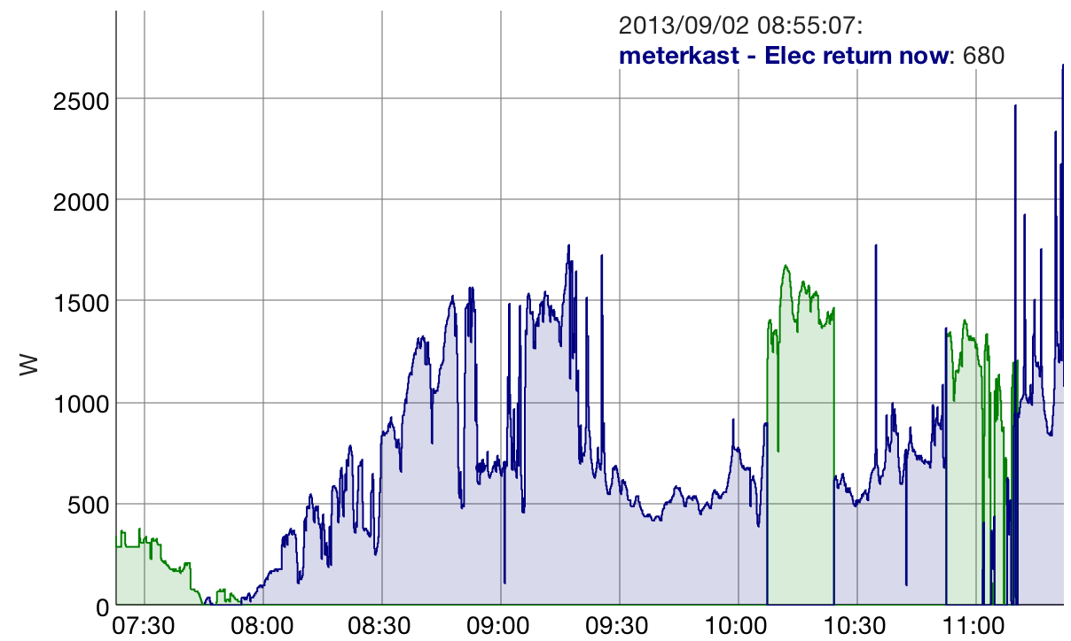
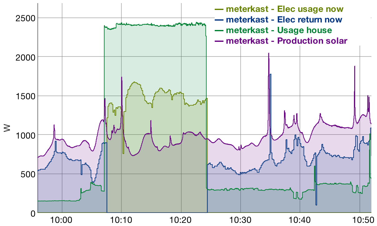
Currently, newReading() does nothing more than turn around and call the show() method of that same data source, which then sends a plain text version of the data out over the serial line. For unattended operation, readings will need to be saved in dataflash memory for retrieval at some later moment.

The above code compiles to 8104 bytes on an ATmega168 so far. Lots of room remaining!

JeeHub prototype

In AVR, Software on Mar 12, 2009 at 00:01

Voilá – the first JeeHub prototype exists!

JeeHub prototype

(click on the image to see the annotated version)

It’s a pretty simple setup so far, as can be seen on the backside:

DSC_0117

All the pieces work, at least in isolation. But the Linux board and the JeeNode haven’t been connected together yet (I need to figure out which serial port to use on the MMnet1001) and there is some strange interaction between the different interrupt-driven pieces on the JeeNode. Looks like both hardware and software troubles at this stage.

Here’s some output:

Picture 1.png

So it’s picking up RFM12B packets, reading external power and battery voltage levels, reading out temperature and barometric pressure, and decoding both the KlikAanKlikUit remote controls and the DCF77 clock signal. But there’s some stuff here which is definitely not kosher – could be interrupt handling issues.

Update – looks like gcc 4.3.0 has trouble with interrupt code. When I changed to 4.3.2, everything started working as expected.

There are also a few hardware glitches in this early prototype, such as the switching regulator interfering with the DCF77 receiver (will change to a linear one) and the 433 MHz radio interfering with the RFM12B (could add some decoupling or shielding).

This first version of the code has been added to the subversion repository.
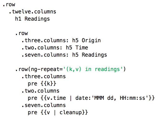
Decoding 433 MHz KAKU signals

In AVR, Software on Mar 10, 2009 at 00:01

Here is a simple OOK receiver, hooked up to AIO port 3:

Decoding 433 MHz KAKU signals

The following interrupt-driven code will pick up signals from a “KlikAanKlikUit” remote control:

Picture 1.png

It should be relatively easy to adapt this to other units. Signals in different protocols can be decoded at the same time, since all decoding state is maintained in a separate state machine.
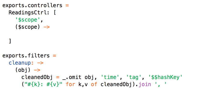
Sample output:

Picture 2.png

The KAKU units use a very crude signalling protocol, with no error checking other than sending a distinct bit pattern for 0’s and 1’s. The sample output has errors, in fact: the B7 after the B6 should have been a B6. It is probably best to only accept commands when they come in more than once in quick succession.

There can be quite a bit of noise from the receiver, in the form of random pulses. These will be ignored, but it may use up some CPU power to service all the corresponding interrupts.

Don't mess with the boot flash

In Software on Mar 9, 2009 at 00:01

Ok, so I tried to get the on-board 4 Mb dataflash of the MMnet1001 working, just out of curiosity…

That was a bad idea. Nothing went wrong for a while, but then I rebooted:

Picture 2.png

And then nothing. Whoops, I messed with the boot partition instead of the dataflash chip! Thankfully, tech support at Propox helped me out quickly. It’s actually quite easy to re-flash the MMnet1001: connect a USB cable to the USB device (not host) port pins, and then simply jump through a few basic software hoops. Neat – well done.

Ah, that looks better:

Picture 1.png

And so on.

So the 4 Mb dataflash remains a mystery for now. No problem, the 1 Gb NAND flash is the main deal, and it works just fine. I’ve added about 7 Mb of my own so far, but that still leaves plenty of free space:

Picture 4.png

The hardware clock works fine, but it needs to be set once before reading it out to get rid of an error message. IOW, set the time zone in “/etc/config/system” (I used “CET-1”), then set the proper date and time with “date”, then finish with “busybox hwclock -w -u”. Note that the “/sbin/hwclock” version doesn’t work for setting the clock (it seems to be ok for readout).

On the software side, I now have a Tclkit build cross-compiled via the OpenWrt SDK and working on the MMnet1001, so the rest of the work can be done on my development system and then copied to this amazing little Linux, eh… box? plug? chip?

Anyway, all is well.

Thank you, Andrzey, for helping out an AT91 newbie ;)

DCF77 clock reception

In AVR, Software on Mar 6, 2009 at 00:01

The DCF radio in Frankfurt sends out a constant beacon signal at 77 KHz which can be received by a cheap radio module all over Western Europe:

DCF77 clock reception

Updatethe above connections are wrong. The diagram was showing the bottom view, all wires need to be flipped over to the other end of the DCF77 screw terminal block. No harm done, it works now.

The code has been added as “dcf77demo” in the Ports library.

Sample output:

Picture 1.png

OOK signaling with an RFM12B

In AVR, Software on Mar 3, 2009 at 00:01

Although the RFM12B was designed for FSK (frequency-shift keying), it can also be used for OOK (on-off keying) transmissions. The trick is simply to turn its transmitter on and off via the SPI interface.

This can be used to control simple RF-controlled devices such as the FS20 power control units by Conrad and ELV in Germany. Here’s a sketch which turns a remote device (lamp, etc) on and off:

OOK signaling with an RFM12B

It turns out that the 868 MHz version of the RFM12B can even transmit 433 MHz signals, at least for simple OOK. The following example turns a device on and off via the low-cost KlikAanKlikUit units sold in the Netherlands, using the same 868 MHz radio module as above:

OOK signaling with an RFM12B

Both demo’s have been added to the RF12 source code library. Other slow-rate bit-stream protocols similar to the above could easily be added.

No attempt has been made to receive OOK signals right now, though one could imagine reading out the RSSI bit to determine the presence of a carrier…

Ports on a standard Arduino

In AVR, Software on Mar 1, 2009 at 00:01

The Ports library described in recent posts works fine with any type of Arduino, Freeduino, etc – not just JeeNodes. It merely uses some conventions for the “DIO” and “AIO” pins of each of the 4 ports.

Here is an example using a HM55B compass module from Parallax, using an Arduino Duemilanove with a Proto Shield from AdaFruit:

Ports on a standard Arduino

There are actually two sensors in the above setup – the bigger sensor is a Parallax H48C 3-axis accelerometer (more on that below). Both need +5V to operate, so they won’t work with simple 4-pin ports on a JeeNode.

Ports are mapped to the Arduino pins as follows:

  • Port 1 DIO = Arduino digital pin 4 (PD4)
  • Port 1 AIO = Arduino analog pin 0 (PC0)
  • Port 2 DIO = Arduino digital pin 5 (PD5)
  • Port 2 AIO = Arduino analog pin 1 (PC1)
  • Port 3 DIO = Arduino digital pin 6 (PD6)
  • Port 3 AIO = Arduino analog pin 2 (PC2)
  • Port 4 DIO = Arduino digital pin 7 (PD7)
  • Port 4 AIO = Arduino analog pin 3 (PC3)

The ATmega register bits are listed in parentheses.

Here is the full code of the HM55B driver plus demo:

Picture 2.png

Sample output:

Ports on a standard Arduino

The H48C 3-axis accelerometer demo is very similar, source code can be found here. Sample output:

Ports on a standard Arduino

These two hookups both use some new utility code in the Ports library to shift a specified number of bits in and out of the DIO line while clocking the AIO line. Note also that these sensors needs two ports each, since they both use 3 IO lines for their SPI-like interface.

All together now

In AVR, Software on Feb 22, 2009 at 00:01

It’s time to combine everything:

Combi demo

This is a setup with all the sensor interfaces documented in recent posts:

  1. a SHT11 to measure relative humidity (and temperature)
  2. a BMP085 sensor to measure barometric pressure (and temperature)
  3. PIR + LDR sensors to demonstrate reading digital and analog signals
  4. a Nunchuk with 2-axis joystick, 3-axis accelerometer, and 2 buttons

A new “combi_demo” has been added to the Ports library. The code is essentially the concatenation of the individual demo source files (you can browse the real thing here):

Combi demo

This example illustrates how the Ports library lets you mix and match drivers and ports at will. Note that two I2C interfaces are running in parallel at different speeds (sure, the BMP085 and the Nunchuk could also have been tied to a single port, running at 100 KHz).

Sample output;

Combi demo

This example compiles to 9114 bytes of code with the Arduino 13 IDE, so there is still plenty of room left to add, say, a wireless driver.

Hooking up a BMP085 sensor

In AVR, Software on Feb 19, 2009 at 00:01

The BMP085 sensor measures barometric pressure (and temperature). I’ve hooked it up to port 2 via I2C:

Hooking up a BMP085 sensor

As SMD, it’s tiny

Hooking up a BMP085 sensor

The 4 wire-wrap wires are connected to port pins 2..5, respectively: SDA (DIO), ground, SCK (AIO), and 3.3V power.

There’s now a bit-banging I2C master driver in the Ports library which works with any of the 4 ports, plus a new driver for the BMP085. Here’s the new demo code, now included with the library:

Hooking up a BMP085 sensor

It looks like the elaborate algorithm from the BMP085 data sheet to calculate pressure in Pascals (millibar) contains an error. After some guess-work and with information from the older SMD500 sensor, I think I’ve come up with the proper computations. The results are now as expected:

Hooking up a BMP085 sensor

This is a very sensitive MEMS sensor. It’s accurate enough in its lowest resolution mode to calculate altitude to 50 cm accuracy given the exact pressure at sea level – just moving the sensor up and down shows a matching variation! Higher-resolution modes have been not been implemented.

Update – There’s a problem with the calculations: with temperatures 25.0 °C and up, the pressure calculations fail and a result of 2.35 mBar is reported. Will need to look into this.

Update 2 – Thanks to a private email suggestion, I’ve finally been able to resolve the > 25 °C bug. The current source code no longer has the problem and shows consistent values also at higher temperatures.

Hooking up an SHT11 sensor

In AVR, Software on Feb 17, 2009 at 00:01

The SHT11 sensor measures relative humidity and temperature. It connects via 2 I/O lines using an I2C’ish protocol with a funny (optional) CRC check. I’ve hooked it up to port 1 on a JeeNode:

Hooking up an SHT11 sensor

There are just four wires to connect to this minute module. Here’s a close-up, with data and ground crossed over to port pins 2 and 3, respectively:

Hooking up an SHT11 sensor

The sensor is mounted free-floating on this little DIY breakout board so it picks up ambient air properties.

A driver for the SHT11 has been added to the Ports library, along with a small demo:

Hooking up an SHT11 sensor

A “sensor” object is defined at the top, tied to a specific “port” – the SHT11 class is derived from the Port class.

Sample output:

Hooking up an SHT11 sensor

The driver uses PROGMEM for the optional crc table. This causes a warning in Arduino-0013 when switching boards (which recompiles PortsSHT11.cpp), probably due to this issue, i.e. gcc bug #34734.

With thanks to Guido Socher for his excellent page about the SHT11 (his version does all calculations using fixed point integers, if you prefer to avoid floats).

Update – Changes checked-in and ZIP file updated. Thanks to Stephen Eaton for pointing out a mistake in the calculation constants for 3.3V.

Remote ports

In AVR, Software on Feb 15, 2009 at 00:07

Yesterday was about local “ports” on the Arduino’ish JeeNode. Today, this is extended to remote ports. Here’s a sketch which controls ports wirelessly:

Remote ports

It’s almost like the local one, except for some headers and declarations at the top and a new “bob.poll()” in the main loop. Where “bob” is defined as the object representing a remote node with id ‘B’ (id’s ‘A’ through ‘Z’ are available for general use). Welcome to the world of messaging and transport independence.

This is a test setup with two JeeNodes:

Remote ports

The receiver (top) is powered by a 3x AAA battery pack (it turns out that 3x NiMh ≈ 4V). The transmitter (bottom) is tied to the USB port. This test sends 25 packets per second through the air (data + ack at 80 msec intervals). Probably OK for a quick test, but not for prolonged use!

This test setup makes it easy to check range by walking around with the receiver. Turns out that it’s just fine for my purposes: this works across 3 stone walls / concrete floors. Data rate is ≈ 57600 baud.

The changes to the Ports library have been included in the new Ports.zip release and in subversion, see also the previous post. Two new examples have been added: blink_xmit and blink_recv. The receiver code decodes and interprets each packet and performs all port I/O requested by the transmitter. Input values are then sent back in the ack packet.

The Arduino-0013 IDE compiles “blink_xmit” and “blink_recv” to 3128 and 2644 bytes, respectively. So there’s plenty of room for more functionality.

Ports library for Arduino

In AVR, Software on Feb 14, 2009 at 00:03

Here is a “Hello world” sketch for JeeNodes, luxury edition:

Ports library for Arduino

It drives 4 LEDs, one connected to each the DIO + GND pins of each “port”. The LEDs on ports 1 and 4 blink at different rates, while LEDs 2 and 3 use the PWM output capabilities to continuously light up and then dim again (like Macs do in sleep mode). Only ports 2 and 3 support PWM.

Here’s a setup using four 4-pin headers on a JeeNode with a mini breadboard (port pins 1 and 6 are rarely used). Note how ports 1 & 2 are rotated 180° w.r.t. ports 3 & 4:

Ports library for Arduino

Each of the LEDs is connected to port pins 2 and 3 with a series resistor. The red LED is port 1, then counter clockwise ports 2 (green), 3 (green), and 4 (yellow). The wireless isn’t being used in this example.

This uses a new “Ports” library which is available as Ports.zip or via subversion. This code needs to be placed in the Arduino IDE’s “libraries/” folder. It includes this “blink_ports” example.

My next post will explain why I went through the trouble of creating this Ports library. For now it’s just a thin wrapper around the standard pinMode(), digitalRead(), digitalWrite(), analogRead(), and analogWrite() calls.
Update – sources now in subversion.

RFM12B library for Arduino

In AVR, Software on Feb 10, 2009 at 00:03

Here’s a driver for the RFM12B radio with Arduino’s and similar AVR boards. The radio is connected as follows:
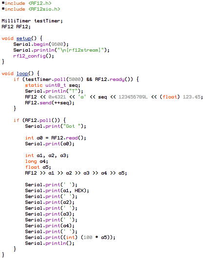
RFM12B

The code is available as RF12.zip or via subversion. It’s packaged as an Arduino library. To try out the included example, you’ll obviously need two Arduino’s + radio modules, connected as above. Then:
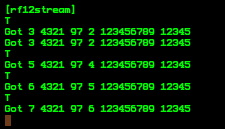
  • unpack the above zip as new directory in your Arduino IDE’s “libraries/” folder
  • build and upload the included example sketch to both systems
  • check proper operation by opening the serial port at 57600 baud
  • you should see a “[RF12DEMO]” greeting on both
  • on one unit, type “0i 0i 1i” to set its node ID to 1
  • on the other, type “0i 0i 2i” to set its node ID to 2
  • send a test packet of 7x <N> bytes by typing “<N>s” (<N> = 0..9)
  • you should see the test packet on the other node
  • use “<N>a” to send a test packet and request an ack

The node ID is stored in EEPROM (the demo uses byte 0), so you only need to initialize ID’s once in each node.

This code uses interrupts to do most of the work in the background for transmission as well as reception. The packet buffer is limited to 66 bytes of data. All packets are verified with a 16-bit CRC.

Packets can be sent to a specific node (ID 1..30) or broadcast to all (ID 0). The demo code sends its test packets as broadcasts, but replies with acknowledgements to just the originator. Note that requesting an acknowledgement for broadcast packets only makes sense with two nodes.

Update – instructions for the demo are now slightly different (see the README).

Ignoring imprecise data

In Software on Feb 9, 2009 at 12:05

For some time, I’ve had a second set of calculations running which produces much more accurate and regular data than some of what’s on these past charts:

Picture 1.png

The difference with the graphs is that only readings which come in exactly at the time the counter changes are considered here. All retransmission (i.e. readings tagged with a late time stamp) are simply ignored. Only one retransmission happens to be in this example (the one marked “6+2”), but it still produces consistent results.

It looks like the gas measurements could be improved by tagging all readings in the sensor node instead of at the receiving end of the packets. That way retransmissions would still be tagged properly, even when readings arrive a bit late.

Hmm, this requires running a clock with milli-second accuracy on the sensor board for best results… not entirely trivial over extended periods of time. The sensor board will need to be synchronized to some other clock – either an on-board DCF77 radio or some data received from another node. And I’ll need to use a crystal instead of a resonator (0.005% vs 0.5% drift).

Still not right

In Software on Feb 8, 2009 at 23:55

The gas measurements are still giving me trouble:

Picture 3.png

I’ve changed scales and plotted all values to better see what’s going on over a small time frame. The electricity consumption looks ok now (these are night-time values). But the gas measurements keep jumping up and down by a factor of around 5 all the time!

Maybe there’s a problem with the sensor readout – there are about 4 readings coming in per minute. Or perhaps the automatic idle transmission of packets every 10 seconds is interfering with this cycle?

I don’t know what’s going on… needs more work!

Measurement anomalies

In Software on Feb 7, 2009 at 02:38

Here’s a more detailed view of the measurement quirks related to gas consumption:

Picture 1.png

The yellowish line is electricity usage, which hovers around 200 watt, while the blue line is the calculated gas consumption. What happens is that the heater cycles on and off approximately once every 15 minutes. When off, no gas is consumed so the meter just stops providing pulses. Then, after roughly 10 minutes it starts again at our heater’s standard rate of around 1.5 m3/hr. If you look very closely, you can see that the “zero” values are actually just above zero. That’s because whatever gas flowed until the rotation stops and whatever gas flows right after it starts all gets averaged-out over the entire period.

What needs to be done, I think, is to re-interpret the long averaged-out period as a period of continued flow at the original full rate, followed by zero flow:

Picture 3.png

I.e. the incoming data was treated as the single-hatched “B”, whereas it should be treated as the cross-hatched bar “A”. Both areas are the same.

Actually, this is not 100% accurate since we don’t know whether the meter stopped near the beginning or near the end of its revolution. But there is simply not enough information in the gas measurement data to disambiguate these cases.

However… as you can see, the electricity consumption also has some surprisingly regular small changes. Those measurements suffer from the same problem, but they have a much smaller impact due the the higher measurement rate. My hunch is that these small wattage changes are actually the electricity consumption of the heater, as it turns on and off!

But hey, who cares for now – these are just instant-by-instant consumption rates. The integral of these rates is the total consumption, and those are by definition “accurate” since I’m measuring the very same metering revolutions which the electricity and gas company use to charge me later on.

Update – Here are the results with the above adjustments:

Picture 1.png

Energy plots

In Software on Feb 6, 2009 at 00:03

And here’s the electricity and gas consumption for (part of) last Wednesday:

Picture 1.png

There are some quirks due to the way things are measured. The meter cannot accurately detect when gas consumption drops to zero, since that simply produces no readings. This can be resolved by adding fake readings when a very low consumption is reported, estimating the times when the gas flow stopped and then started again.

The electricity peaks at 19:45 are from the induction stove, the one around 20:15 is probably the close-in boiler.

This Tcl code generates the necessary HTML/JavaScript snippet to produce the plot:

Picture 3.png

All measurement data selection is handled by the “dataset loop” command, which takes a measurement parameter name, the selection range, and the names of the time and value variables to set during the loop.

Temperature graphs

In Software on Feb 5, 2009 at 13:30

Some weather & energy data has been coming in over here for over a month now, logged to text files, and patiently awaiting further processing. Here are the results of a few days of hacking around on the software side of things:

Picture 1.png

This is a test page served by a custom web server, with all data now stored in a database. I’ve used several bits of software which are dear and near to me:

  • the database used is my own trusty Metakit
  • the custom software is written in Tcl
  • the web server is based on my Rig modules
  • the plots are generated in the browser by Flot
  • it’s all in two files using using Tclkit / Starkits

The code is portable and works on Mac OS X, Windows, and Linux. The system requirements are minimal, so it runs just fine on my NSLU2 and Bubba NAS boxes.

Things are starting to come together nicely…

16 x 8 LEDs

In AVR, Software on Jan 30, 2009 at 21:51

Here’s the umptieth LED board:

DSC_0039.jpg

It’s been hooked up to SPI and FTDI connectors, and the two 8×8 LED matrices have been tied to an ATmega168 and an A6276 chip, described as a “16-Bit Serial Input, Constant-Current Latched LED Driver”. The voltage regulator and the I2C/power pins on the right haven’t been hooked up yet.

This shows the backside, which is surprisingly robust once done, but a huge pain to build:

DSC_0040.jpg

I use wire-wrap wire because its insulation can stand the soldering heat without problems and because the wire bonds easily with solder. For anything but one-offs, pcb’s are obviously a much better way to go.

Here’s the unit hooked up via a USB/FTDI board by ModernDevice:

DSC_0042.jpg

Here’s a better view with one LED actually turned on:

DSC_0044.jpg

The brightness and contrast are actually far better than in the above picture.

The design is made for scanning across columns while providing 8 bits of on/off data for the current column via 8 output pins on the ATmega. There’s a 16 MHz resonator on board, so this thing is fully compatible with the Arduino IDE.

Here’s a sketch which makes a single led turn on and meander across all positions:

Picture 1.png

This was used to verify that each dot is accessible and that there are no short circuits. The analogWrite() call is used to vary the display brightness, by controlling all LED driver outputs via PWM. Another useful property of this driver chip is that it needs only one resistor to limit the current through each of the leds.

Update: Silly me, with constant current on the columns, I have to cycle the rows of course. Will need to add an ULN2981 driver to allow the row pins from the ATmega to drive up to 16 leds at once. With this change the LEDs will cycle at 125 i.s.o. 62.5 Hz and can be slightly brighter.

Reliable comms with RFM12B

In AVR, Software on Jan 23, 2009 at 16:34

The driver code for RFM12B radio modules is starting to shape up nicely. It’s all interrupt-driven, so it works mostly in the background. Here’s a complete sketch for Arduino, allowing bi-directional sending of test packets with or without acknowledgement:

Picture 1.png

Most of this logic is the test code itself. The main interface calls are:

  • rf12_initialize() – call this one in setup()
  • rf12_recvDone() – returns 1 when a complete packet has been received
  • rf12_canSend() – call this to start sending when possible
  • rf12_sendStart(hdr,buf,len) – this starts actual transmission

All the interrupt stuff happens behind the scenes, the only requirements being that rf12_recvDone() should be called frequently and that rf12_sendStart() may only be called after rf12_recvDone() or rf12_canSend() return true, i.e. inside the above if statements.

The driver itself is under 200 lines of C code, it’ll be released as open source once the code settles a bit.

A simple RF pulse scope

In AVR, Software on Jan 10, 2009 at 23:45

Here’s a simple way to analyze RF pulse trains, as emitted by simple 433/868 MHz remote controls. A receiver for the proper frequency band is required, as well as some Arduino board connected to USB.

The code is a sketch which picks up all 0/1 transitions (i.e. presence/absence of the radio carrier) and reports the elapsed time between each transition:

Picture 1.png

The radio signal is tied to the analog comparator (pin 7), and the timer is set to count in 8 µsec steps. This rate was chosen to allow for pulses up to 2 msec.

The data is sent as a stream of bytes. Values 2..255 correspond to pulse durations of 16..2040 µsec. A “0” is sent for longer breaks, a “1” is sent if the data was not transmitted fast enough over USB, i.e. an overrun. Note that “0” values are only sent once, i.e. when there is no signal no bytes are sent to the USB interface.

On the computer side, all sorts of software could be used/written to analyze these pulse trains. I used Tcl for a one-off analysis of KlikAanKlikUit remotes operating at 433 MHz, though it would be really neat to have some sort of logic analyzer GUI or web interface added to this.

Transmit via interrupts

In AVR, Software on Jan 8, 2009 at 16:37

Making the transmit logic of an ATMega MPU with RFM12B radio module interrupt-driven is not very hard, as it turns out. The idea is to use states to decide what to do when a new transmit interrupt comes in. These are the states I’m using:

Picture 1.png

And this is the interrupt handler:

Picture 2.png

Lastly, this code starts a new transmission (assuming txstate was TXIDLE):

Picture 3.png

The main trick used in the above is that the state usually increments on each interrupt and that negative states are used to send all the payload data bytes. So the choice of state values matters, i.e. TXCRC1 has to be zero.

More readings

In Software on Dec 19, 2008 at 15:55

Here is the latest display showing on my screen:

7474AFF5-C9D3-4DA7-B5E3-492EE65C15DB.jpg

Updated in real time, with new readings coming in every few seconds for electricity and gas and every few minutes from the weather station (still sitting here in the office for now, so the values are bogus).

Good RF with RFM12B

In AVR, Software on Dec 11, 2008 at 15:38

Yippie. Got a simple blinking LED demo running on RFM12B’s after lots of head-scratching. Had to understand ATmega’s SPI mechanism to get there, but these two boards now talk to each other over the air, uni-directionally:

Good RF

That’s an Arduino Mini Pro (which runs at 3.3V internally, as does the RFM12B). Power comes from the FTDI cable, but with a special hack to drive the raw power input from it, not the default VCC connection. This way, the on-board 3.3V regulator is used to lower the voltage for both the MCU and the wireless module.

The other board is a bit of a mess, has the same Mini Pro, but some other stuff which is partly a left-over from earlier experiments:

Good RF

Here a USB interface is used to provide 3.3V power. It’s functionally identical to the first board: with RFM12B’s the same setup can be used as transmitter or as receiver.

The top board is the receiver – its picture shows the green LED on, i.e. correct packet reception!

The hookup is very simple, just 5 wires between RF module and MCU, and 2 power pins / 1 pull-up / 1 antenna wire on the RF module is all it takes. The 5 wires are standard SPI plus an IRQ line:

  • MOSI (MCU) –> SDI (RFM)
  • MISO (MCU) <– SDO (RFM)
  • SCK (MCU) –> SCK (RFM)
  • SS (MCU) –> nSEL (RFM)
  • PD2 (MCU) <– nIRQ (RFM)

It took some work to get the software working. The trouble with this stuff is that until you get both transmitter and receiver working properly, it all remains a bit hard to debug. And there are quite a few registers to set up on the RFM12B to make it do its magic.

But after some tweaking, the rfm12xmit and rfm12recv sketches for the Arduino IDE started working. First with bit-banged SPI coding, but then also with the ATmega168’s built-in SPI hardware. Which is nice, because all exchanges now take place at 1..2 MHz (i.e. 8..16 µsec per 16-bit command). All I/O with the RF module uses simple busy polling for now.

The RF range and quality of reception with the RFM12B is considerably better than my earlier 868 MHz AM setup. Packets now easily get across 3 layers of stone/concrete and all of them appear to be arriving properly.

Update – here’s the C source code for the xmit and recv sides.

Update 2 – the connections for MISO and MISO as listed above were reversed – many thanks to José Xavier for pointing this out. The text above has been fixed.

Timer Interrupts

In AVR, Software on Dec 6, 2008 at 15:33

Here is some new interrupt-driven receiver code. This receiver is considerably better at identifying correct packets, regardless of what other bit patterns are coming in. The new code is based on a state machine which takes pulse times and gaps into account, detecting all valid sequences of pulse widths and rejecting all outliers. The main code is:

AA4D1C74-E3E3-41B7-BD67-90E432711496.jpg

Then, in the main loop, this code picks up the results:

EFC8BB55-ECC5-4553-9C8D-17CB1F9A92CC.jpg

Also, with an interrupt driven design the receiver no longer depends on timing loops and is free to spend its time in other logic. It is now possible to run multiple state machines in parallel, decoding a variety of different signal patterns.

Success @ 868

In AVR, Software on Dec 3, 2008 at 15:29

As expected, a lot of the bit-level reception problems with the 433 & 868 MHz wireless issues can be resolved with better packet framing and reception logic. Here’s part of the latest reception log, alll the way across those elusive 3 stone/concrete walls:

93E74FE4-4BB6-4209-A2EE-7700D52833DF.jpg

There are still times when proper reception stutters, but as long as reception recovers within a minute or so that’ll be fine for the purpose of low-rate data logging.

The send format now includes an old-fashioned SYN-bytes-plus-SOH header:

176528F4-75FD-4BB2-B7CA-5CF5EA7105A9.jpg

Reception takes a bit more code, here’s the basic frame reception loop:

86C83486-9950-4FB9-B4BE-8D5FB482ED49.jpg

And here’s the bit-level decoder:

23F292A5-C471-4C4E-A654-96D7A5E10263.jpg

The receiver + serial debugging code takes a mere 3208 bytes so far.